Image classifiers do not always look where we expect. One well-known model recognised horses by a photographer’s copyright tag in the corner of the frame, and only a map of the pixels it relied on revealed the shortcut. Layer-wise relevance propagation (LRP) is a classic way to draw such maps. On modern vision models, however, it can fail without warning, producing either noise or maps that look plausible while carrying the wrong amounts.
This post shows why and fills in the missing rules, which come with a companion notebook.
What is relevance?
A deep network passes an image through a stack of layers until the last one makes the prediction. We can view each layer as a separate network in its own right, which takes an input, computes an output and passes it to the next layer. Now think of the output of the whole network as water that we pour back through it. At every layer, the water held by each neuron is divided among the neurons that fed into it, and a neuron that contributed more receives more. To know how much each one contributed, we store the intermediate outputs during the forward pass and reuse them on the way back. Whatever reaches a pixel tells us how much that pixel contributed. This water is called relevance, and the procedure is layer-wise relevance propagation [Bach et al.]. Spread over all the pixels, the relevance forms a heatmap, and a heatmap like this is what caught the horse classifier reading a copyright tag [Lapuschkin et al.].
The figure below runs LRP on a small network that reads handwritten digits. Its forward half computes the prediction, and its backward half passes the score back to the pixels. You can draw your own digit on the input.
This figure needs JavaScript.
Notice how the two halves mirror each other. The backward pass walks the same path as the forward pass, only in the opposite direction, and at every step it relies on what the forward pass stored there to split the relevance. The relevance usually starts with the score of the class being explained, but here it starts with 1.00. Since relevance is only redistributed and never created, the number under each column stays at 1.00 from layer to layer. This property is called conservation. Starting at 1.00 only rescales the numbers and leaves the maps unchanged, yet it makes conservation easy to check, since any relevance that leaked out or appeared from nowhere would pull a column away from 1.00. Hover over a neuron on the right, or tap it, to see how much relevance it holds and where it flows on its way to the pixels.
How we distribute this relevance is decided by a rule, and each kind of layer needs one that fits what it computes. The figure uses the $z^+$ rule, which follows only the contributions that raised the score. It cannot say what pulled a score below zero, so for a class with a negative score the figure starts with 0 and shows an empty map. Choosing these rules well is most of the work, and Layer-Wise Relevance Propagation: An Overview describes the common ones and when to use them [Montavon et al.].
Relevance is not a gradient
Most explanation methods for neural networks are built on the gradient, but the gradient answers a different question than relevance. A single neuron is enough to see the difference. Take one with inputs $x_1 = 2$ and $x_2 = 1$, and weights $w_1 = 1.5$ and $w_2 = -1$. It multiplies each input by its weight and adds the results, so it outputs $3 - 1 = 2$. The gradient asks how sensitive the output is to a small nudge in each input, and for this neuron the answer is simply the weights, 1.5 and −1.
The figure below shows this neuron. Like the digit network, it is mirrored around the output. Drag the inputs and the weights on the forward side, and the relevance flows back to the inputs on the other side, red for positive and blue for negative.
This figure needs JavaScript.
Relevance asks instead how much of the output came from each input. An input contributes its value times its weight, so $x_1$ contributed 3 and $x_2$ contributed −1, while an input of zero would contribute nothing, however large its weight. LRP divides the relevance that arrives in these proportions, and this basic rule is called LRP-0. Starting from the output of 2, it passes 3 back to $x_1$ and −1 to $x_2$, so the input that worked against the output receives negative relevance, and the total stays 2. The $z^+$ rule of the first figure follows only the positive contributions, with $z$ for a contribution and $+$ for its positive part. It gives all of the 2 to $x_1$ and nothing to $x_2$, so relevance never turns negative. Since every layer is made of such neurons, repeating this step layer by layer carries the relevance all the way to the pixels.
In code, LRP runs on the same backward pass that computes gradients, and each rule overrides how its layer passes values back. A layer without a rule raises no error and simply multiplies the incoming relevance by its gradient, here $1.5 \times 2 = 3$ and $-1 \times 2 = -2$, which adds up to 1 instead of the 2 that arrived. We will call this the gradient fallback, and it is behind every failure in this post. The switch in the figure above shows it for any inputs and weights.
The next figure compares the two on the digit network. With the gradient, the total changes from layer to layer and some values turn negative, shown in blue. The pixel map also reaches into the empty background, which contributed nothing to the score. With LRP, every column holds the same total and the background stays empty.
This figure needs JavaScript.
The second switch decides whether to keep negative values, giving four methods in total. The plain gradient is ordinary backpropagation, the same backward pass that trains the network, and its pixel map is known as a saliency map [Simonyan et al.]. LRP-0 and $z^+$ are the two rules from our single-neuron example. Guided backpropagation is the gradient’s counterpart to $z^+$, passing back only the positive part of the gradient, yet some blue remains and the totals still change. You can hover over the classes to compare them.
What is guided backpropagation?
Guided backpropagation was introduced to produce sharper pictures of what a convolutional network responds to [Springenberg et al.]. It runs ordinary backpropagation, but at every neuron it keeps only the positive part of the gradient, and only if that neuron was active in the forward pass. This filtering happens at the neurons, so multiplying by negative weights on the way to the previous layer can create new negative values. Inside the network, the next set of neurons drops those negative values again, but the input pixels have no neurons to filter them out, leaving some blue in the final heatmap. Since it still multiplies by the weights instead of dividing a fixed share, the totals change from layer to layer.
The two LRP rules treat the classes differently. Since LRP-0 keeps negative contributions, we can explain a class with a negative score by setting its starting relevance to −1. In the figure above, this produces a distinct map for each class. The $z^+$ rule follows only positive contributions, so it starts at 0 when the score is negative. Even for another class with a positive score, using $z^+$ in every layer produces almost the same map as for the prediction, because without negative contributions the backward pass depends mostly on the input and hardly on the class. For that reason, the figure shows the $z^+$ map only for the predicted class and sets the rest to 0.
The first attempt
The previous post applied LRP to self-supervised vision encoders, which learn from images without any labels. Instead of a score for each class, such an encoder turns an image into an embedding, a vector of numbers that describes the whole image. Inside, it computes a feature vector for each cell of a coarse grid over the image, and the embedding it outputs is simply their average. The relevance can therefore start from these features directly. Only their positive part is used, scaled to add up to 1 as in the digit figures.
What are features, and how does the relevance start from them?
What a feature vector stands for depends on the architecture. For a $224 \times 224$ image, a vision transformer (ViT) cuts the input into patches of $16 \times 16$ pixels and turns each patch into a feature vector, called a token. Its grid therefore has $14 \times 14$ cells, and attention lets every token draw on the whole image. In a convolutional network, each feature vector on the grid summarises a region of the image called its receptive field, which grows with every layer. Hierarchical models like ConvNeXt, Swin, and MaxViT shrink the image in stages to a grid of $7 \times 7$ cells. Each feature vector holds several hundred numbers, called channels, for example 768 in ViT-B and 1024 in ConvNeXt-B.
Each positive number in the grid, one for each cell and channel, starts with its value divided by the sum of all positive numbers across the grid, while negative numbers start with 0. The starting relevance then adds up to 1, and whatever arrives at the pixels is the share that made it all the way through. Since the features add up to different totals in different models and images, this scaling also makes the numbers comparable across all of them. We get the exact same result if we start at the pooled embedding, give each channel its share of this positive sum, and pass the relevance back through the averaging layer with the $z^+$ rule.
Only the positive part is used because the features of most modern encoders are signed, so starting from the raw values would let positive and negative numbers largely cancel out. In ConvNeXt, Swin, and plain ViTs, the raw sum of all feature values retains only 1 to 5% of their total magnitude, and for several of these models the sum is negative on almost every image. ResNets do not have this problem, because their features pass through a ReLU and are never negative. Taking the positive part avoids this cancellation and gives zero or negative features no relevance at all.
To see how LRP behaves on modern architectures, we will test encoders across the current design space: ConvNeXt (a modernised convolutional network), the plain Vision Transformer (ViT), masked autoencoders (MAE), Swin, which restricts attention to local windows, and MaxViT, a hybrid that mixes convolutions with attention. All of them do most of their work in convolutions and fully connected layers. Both simply multiply each input by a weight and add the results, so we will call them linear layers. Two PyTorch libraries already provide ready-made LRP rules for them and for several surrounding operations. zennit covers classic convolutional networks such as VGG and ResNet [Anders et al.]. Instead of editing the model’s code, it attaches rules to the layers while an explanation runs, and restores it afterwards. LXT, the implementation of AttnLRP, covers language models and the original vision transformer [Achtibat et al.].
Why not simply use zennit or LXT?
Both libraries have rules for linear layers, and these carry over to the encoders here. However, zennit has no rules for LayerNorm or attention. LXT does have rules for LayerNorm, GELU, and attention, but it relies on custom model implementations written for a few specific architectures. The encoders we use here come from the timm library, which defines these blocks with its own code. We therefore implement the missing rules in zennit’s way, attaching them directly to the existing layers.
So we start where the libraries stop, with the usual rules for the linear layers and no rule for anything else. The first column of the figure below shows the result for three encoders, and in all of them the map is noise.
Dog and cat1 / 5
How to use this figure
Pick an image from the dock and compare the columns across a row. Each row is one model. The number under a map is how much of the starting amount of 1 arrives at the pixels.

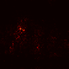
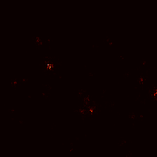

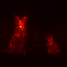
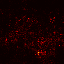

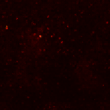
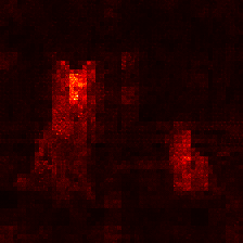
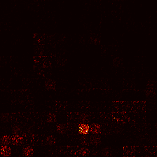
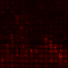
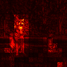
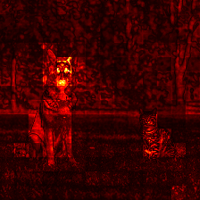
The maps show the positive part of the relevance, while the number under each map is how much of the starting relevance of 1 arrives at the pixels. In the first column, that total ranges from almost nothing in ConvNeXt to more than a thousand in the DINOv1 ViT, and neither is possible when relevance is only redistributed. Every part without a rule fell back to the gradient. The two middle columns each add a single rule, and the last column has all of them. Even there, the total falls short of 1, not because a rule is missing, but because part of the relevance stays inside the network, as we will see shortly.
The missing rules
Beyond their linear layers, these models rely on five operations that off-the-shelf LRP libraries leave uncovered here, namely residual connections, LayerNorm, GELU, layer scale, and self-attention. To see what each missing rule does, the toy ConvNeXt example below has the same parts as the real encoders, and its switches choose between the rule and the gradient fallback for each one. You can also select any block in the diagram to inspect how the relevance flows through it.
This figure needs JavaScript.
What each operation in the block does with the relevance
Residual connections
In a plain network, each layer passes on only its own output. Modern networks wire skip connections around each block of layers. A residual connection is a skip that carries the input of a block forward and adds it to the block’s output, which we call the update. Each block thus computes only a change to its input. The running sum that passes from block to block carries the input along with every change added to it and is called the residual stream.
On the backward pass, the addition at the end of each block causes relevance to multiply when we fall back to the gradient. The gradient of an addition is 1 for both inputs, so the fallback hands the full relevance to the skip and another full copy to the update, doubling the total at every block as shown in the toy ConvNeXt example above.
A real ConvNeXt has 36 residual connections in a row and a ViT has 24, so the copies pile up from block to block. In the third column of the gallery above, LayerNorm already has its rule, but every residual connection copies the relevance. As a result, 450 thousand times the starting relevance reaches the pixels in the DINOv1 ViT, 720 times in ConvNeXt, and almost three trillion times in Swin. Each map is scaled to its own maximum, so none of this shows visually, and in the DINOv1 ViT the objects even look right. The fix is to replace the gradient at every addition with a rule that divides the relevance between the two branches in proportion to the share each contributed.
LayerNorm
On the forward pass, every block adds its output to a running residual stream, so the numbers steadily grow. Left unscaled across dozens of blocks, those accumulated sums would dominate the smaller updates computed by later layers. Each block therefore passes its values through LayerNorm, which subtracts the mean at each position and divides by the spread. That resets the numbers to a standard scale, centred at zero with a spread of one, before the next layer reads them.
That normalization creates a trap on the backward pass. LayerNorm only tracks how far each input sits from the group average. Increasing every input by the same amount raises that average to match, leaving every distance unchanged and producing zero effect at the output. As we saw on the single neuron, a gradient measures how small input changes affect the output. When shifting every input together produces zero effect, the individual gradient values must cancel out and sum to zero. The gradient fallback therefore splits whatever relevance passes back into positive and negative parts of nearly the same size, as the LayerNorm card under the toy ConvNeXt example shows.
A real encoder has a LayerNorm in every block, so this happens dozens of times on the way to the pixels. Whether a channel turns negative depends on how its value compares to the group average. Once the relevance reaches the input, opposing signs may land on neighbouring pixels or largely cancel out, making the resulting map uninformative. The second column of the gallery from the first attempt shows this, even though every residual connection there already divides the relevance properly. The totals expose that failure, ranging wildly from 0.01 in ConvNeXt to millions in Swin.
The fix is to treat the spread as a constant on the backward pass, while keeping the forward pass exactly the same. LayerNorm then behaves like a linear layer, and relevance passes through it with the default rule. Conservative propagation proposed this treatment for transformers [Ali et al.], and AttnLRP uses an equivalent rule [Achtibat et al.]. Looking at the third column, this rule alone brings out the objects in the DINOv1 ViT, though with the inflated totals of the copying residual connections, while ConvNeXt and Swin stay noisy. Only the last column, with all rules in place, displays the objects cleanly across all three models with a plausible total.
GELU and layer scale
Two linear layers in a row act like a single one, meaning the model can only compute weighted sums of its inputs. To break that linearity, an activation function sits between them and acts like a selective gate on each individual value. ResNet uses ReLU, which blocks negative values by setting them to zero. Transformers and ConvNeXt use GELU, a smooth cousin of ReLU that lets small negative values pass through. Alongside activations, these blocks often use layer scale, which multiplies each channel of a block’s output by a learned number before it joins the residual stream.
Both GELU and layer scale act on each number individually. Since each output depends on a single input, relevance passes straight through them unchanged, which AttnLRP calls the identity rule. The gradient fallback instead multiplies the relevance by the slope of GELU or by the learned numbers of layer scale. For the small negative values that GELU lets through, that slope is near zero or even negative, so their relevance mostly vanishes or flips its sign. Layer scale distorts the backward signal in much the same way, shrinking some channels, boosting others, and flipping the sign of a few.
In zennit, the identity rule is applied to every standard activation function, but timm implements GELU with a custom class that zennit fails to recognise, falling back to the gradient silently. In ConvNeXt with the rule, 0.66 of the starting relevance reaches the pixels, and without it only 0.48, so about a quarter is lost on the way. Yet the two maps look the same.
Attention
Transformer blocks replace convolutions with self-attention. A vision transformer divides an image into patches and encodes each patch as a feature vector called a token. In an attention layer, every token updates itself by taking a weighted average of all tokens. Unlike the fixed parameters of a linear layer, these attention weights are probabilities computed dynamically for each image via softmax.
A token’s true contribution to that average is the token multiplied by its attention weight. Under a standard gradient fallback, the backward pass splits into two paths. Along the token path, relevance flows strictly in proportion to the attention weight, ignoring the magnitude of the token itself. Along the attention path, gradients flow back into the softmax computation that produced those probabilities.
Softmax converts raw similarity scores into probabilities that sum to 1, acting as a soft version of argmax. With the attention weights summing to 1 and the attention-path gradients splitting into positive and negative amounts that cancel to zero, a missing attention rule still conserves total relevance. It routes that relevance by attention weight instead of true contribution, doing far less harm than a missing rule for LayerNorm or the residual connections.
Freezing the attention weights during the backward pass corrects this routing. Treated as fixed constants, they receive no gradients and act like the static weights of a standard linear layer, routing relevance by true contribution, where each token is multiplied by its attention weight. This strategy defines conservative propagation [Ali et al.]. AttnLRP goes further by introducing dedicated propagation rules for the attention-weight computation itself, improving faithfulness on image classifiers [Achtibat et al.]. In our encoders, freezing the attention weights changes the maps only slightly. The figure below demonstrates this on a toy example with three tokens: the total stays the same under all three rules, while each token receives a different amount of relevance.
This figure needs JavaScript.
Smaller pieces
A few smaller parts needed a rule as well. MaxViT scales its channels with gates that it computes from the input itself, a design called squeeze-and-excitation. The rule holds these gates constant on the way back, so relevance passes through them unchanged, as with layer scale. Batch normalisation, used in older networks, can be folded into the convolution before it, which turns two layers into one without changing the forward pass. Such rewrites of a model are called canonization [Motzkus et al.]. Folding is only exact when the convolution feeds nothing else, so the code checks that before merging.
Where the relevance goes
With a rule for every part, the maps make sense again, and we can follow the relevance on its way through the network. The figure below does this for seven encoders. Each row starts on the left with the final-layer features and tracks the relevance step by step toward the input pixels on the right.
Dog and cat1 / 5
where it starts
the features
This figure needs JavaScript.
The encoders differ in how far the relevance moves on its way. A convolution only combines neighbouring cells, so in ConvNeXt the relevance stays close to where it started, and about three quarters of it lands on the starting cell and its eight neighbours. Attention connects every token with every other one, so in a ViT the relevance can jump across the image within a single block. In the DINOv1 ViT, only 40 to 50% stays this close.
ResNet-50 adds a pattern of its own. In its middle stages, one cell in every $2 \times 2$ square holds 60 to 70% of the relevance, imprinting a fine checkerboard that has nothing to do with the image [Odena et al.]. It comes from the downsampling shortcut when a stage halves the spatial resolution. The $1 \times 1$ shortcut steps by two cells at a time and reads only one cell in every $2 \times 2$ square, so on the way back the relevance can only return to the cells that were read. By the time it reaches the pixels, the pattern has evened out.
MAE behaves differently, even though it is a ViT as well. Like DINOv1, it starts with relevance spread almost evenly over the image. DINOv1 gathers it onto the objects on the way back, but MAE keeps 70 to 80% on the starting cell and its neighbours, so its maps stay nearly flat at every depth. If we select a single cell on the dog, a faint trace of the rest of the animal appears, far weaker than in DINOv1.
At the pixels, MAE adds a second oddity. A fine grid traces the border of every patch, and about 70% of the relevance lands within two pixels of a border, in a strip that covers only 44% of the image. In DINOv1, the same strip receives a share in line with its area. Since each patch still passes on exactly what it received from the layer above, the grid must form in the very last step, where the first layer spreads a patch’s relevance over its pixels.
In DINOv2, a few dark cells in the background start with much less relevance than the rest. They belong to outlier tokens, a known quirk of some ViTs [Darcet et al.], and they fade within a block or two without leaving a trace at the pixels.
The plain ViTs, whose maps are the most scattered, have something else in common. ConvNeXt, ResNet-50 and Swin learned from labelled images, while the DINO models and MAE were trained in label-free settings. A supervised model only needs the features that tell its classes apart, so it may learn to ignore much of the background. A self-supervised model has no labels to tell it what matters and may keep features of everything in the image, which would spread the relevance more widely.
A scattered or flat map is not necessarily noise, though. As discussed in the previous post, every map in the figure adds up all the features at a position into a single number, so it shows where the relevance lands but not what it stands for. Relevance on the grass and the trees may come from features that describe the background as well as others describe the dog. Once the features are added up, a map has no way to say which is which.
Where the rest of the relevance goes
How much relevance arrives differs a lot between models, from 0.03 in ResNet-50 to 0.69 in Swin for the dog and cat. The rest stays inside the network. Most layers add a constant, the bias, to their output. The bias is not an input, yet part of the output is due to it, so the rules leave part of the relevance with it, and small stabilising terms in the rules keep a little more. In transformers, the class token and the register tokens, extra tokens that the model learns and adds to the patch tokens, take their share as well.
A bias can even hold a negative share. The final normalisation of DINOv3 adds a bias to each feature, and over the features where the relevance starts, these biases add up to a negative amount. The features were therefore larger before the bias was added, so the tokens below receive 5 to 11% more relevance than the start, and the bias keeps the difference as negative relevance. Counted together with the bias, the total is still 1.
Is this a flaw? AttnLRP argues that it is not. Following the original LRP paper, it treats a bias as an extra input whose value is always one, so that its relevance is “preserved, rather than lost” [Achtibat et al.]. One could force all relevance onto the pixels, either by spreading the bias’s share over the inputs or by leaving the bias out of the rules, but AttnLRP warns that spreading can make the results numerically unstable and that leaving out the bias can flip their signs. Leaving out the bias kept all of the relevance in a ResNet but produced invalid numbers in ConvNeXt with the rules used here. This post therefore leaves part of the relevance inside the network and reports how much reaches the pixels.
Position embeddings are the one place where the error goes the other way and too much reaches the pixels. Most ViTs add them to the patch tokens with a plain addition that has no rule here, so its gradient hands the full relevance to the patches, including the share that belongs to the positions. Bakish et al. show that position embeddings carry relevance of their own and that ignoring them violates conservation [Bakish et al.].
Choices that remain
Once the rules are in place, three choices are left. They decide how the relevance is split at each residual connection, which rule the linear layers inside the blocks use, and how the first layer spreads relevance over the pixels. None of them breaks the maps, but each one changes them.
Who gets the credit at a residual connection
A residual connection with a rule must still decide how much of the relevance goes to the skip and how much to the update. There are several reasonable answers, and they behave very differently.
- An equal split gives each part half, regardless of the numbers.
- A proportional split gives each part the share it contributed. This is the standard LRP treatment of an addition, and it is what LXT and AttnLRP do implicitly. A part that worked against the sum receives negative relevance.
- A magnitude split divides by size and ignores the sign. The code uses it for MaxViT and the ViTs, because the proportional split made some of their maps unstable in early experiments.
- A $\gamma$ split works like the proportional one, but gives extra weight to the part whose sign agrees with the sum [Berend et al.].
The proportional, magnitude, and $\gamma$ splits agree as long as the skip and the update have the same sign. They part ways when the update works against the skip. The proportional split then gives the update a negative share, which records that it pulled the sum down. But when the two almost cancel, this split divides by a sum close to zero and hands out huge amounts of both signs. The magnitude split ignores the signs and so avoids this blow-up, but it credits the update as if it had helped. The $\gamma$ split takes the middle way. It keeps the update’s negative share but gives extra weight to the part that agrees with the sum, so the two can no longer cancel out and the amounts stay small. Berend et al. see this kind of cancellation inside transformer blocks as a main reason why LRP maps of ViTs turn noisy.
Dog and cat1 / 5
How to use this figure
Pick an image, then compare the four splits across a row. Each row is one model, and every other rule stays the same.
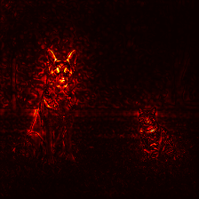
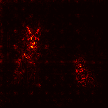
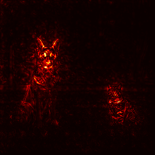
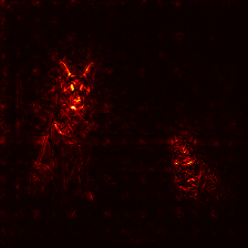
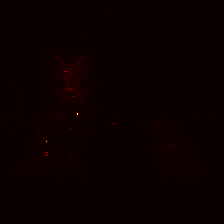
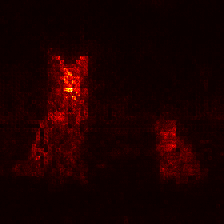
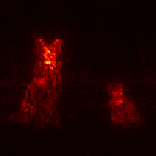
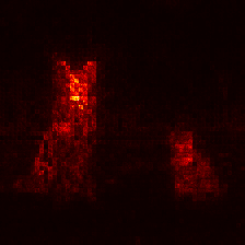
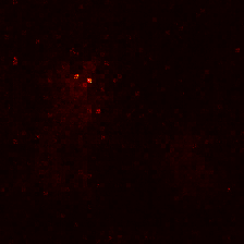
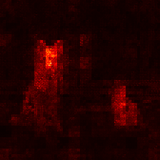
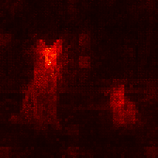
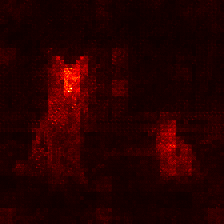
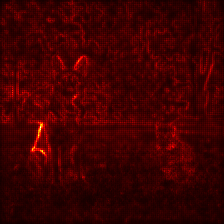
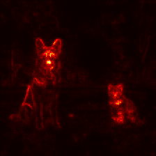
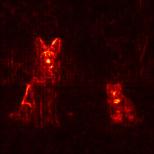
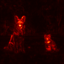
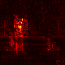
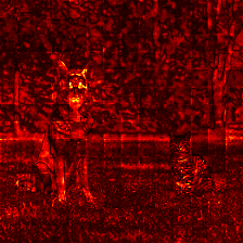
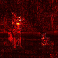
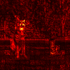
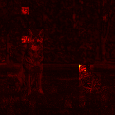
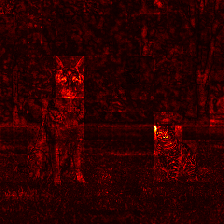
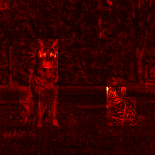
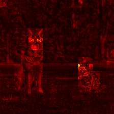
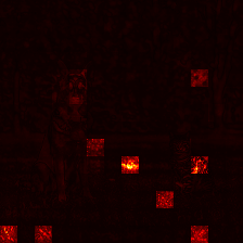
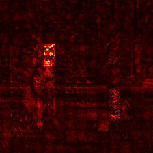
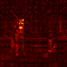
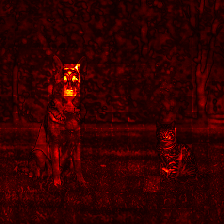
In the maps, the equal split stands out first. In a deep network, it sends half of the relevance into every block’s update, where part of it stays behind with the biases, so very little reaches the pixels, about 0.04 for the DINOv1 ViT and less than 0.001 for MaxViT. The proportional split delivers the most relevance, but in DINOv1 it also spreads it over the grass and the trees, while the magnitude and $\gamma$ splits keep more of it on the animals. Of these two, the $\gamma$ split passes on more relevance and is a little more detailed.
We can choose a split by looking at maps like these and by checking that small changes to the input do not change the maps much. Which split is more faithful to the model remains untested here, and a handful of images would not be enough to claim one. For anyone who wants to choose between them, Berend et al. compare the $\gamma$ split with the standard rules on several faithfulness measures, which test whether the pixels a map highlights are the ones the model actually depends on.
The rule inside the blocks
The linear layers inside the blocks had a rule from the start, but zennit offers several, and they trade detail against focus. Apart from ResNet-50, the encoders here use the Gamma rule, which lies between LRP-0 and the $z^+$ rule. Like LRP-0, it keeps negative contributions, but it gives the positive ones extra weight, and the larger its parameter $\gamma$, the closer it comes to $z^+$. This makes the maps less noisy, and AttnLRP recommends it for the linear layers of vision transformers [Achtibat et al.].
The last step to the pixels
The first layer of many modern encoders cuts the image into patches and turns each patch into a feature vector, $4 \times 4$ pixels in ConvNeXt and Swin and $16 \times 16$ in a ViT. Its rule decides how a patch’s relevance is spread over its pixels, and with that, most of the fine detail in the map. Several rules in zennit can handle this step, and it is not obvious which one suits a patch layer.
- $z^+$ splits a patch’s relevance by how much each pixel pushed the layer’s output up, as in the digit network.
- WSquare splits it by the weights alone, so the image itself plays no part. It is recommended for inputs without natural bounds [Montavon et al.].
- Gamma also counts the pixels that pushed the output down, but favours those that pushed it up. It is the rule the encoders already use for their linear layers deeper in the network.
WSquare ignores the pixels, so it fills every patch with the same pattern, scaled by the patch’s relevance. In the DINOv2 and DINOv3 ViTs, this one repeated pattern accounts for more than 99% of the detail within the patches. $z^+$ follows the image inside each patch instead, which is why it is the first-layer rule for the ViTs.
Dog and cat1 / 5
How to use this figure
Pick an image and compare the three rules for the first layer across a row. Each row is one model, and everything above the first layer is identical. Move the pointer over a map to see the image underneath.
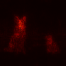
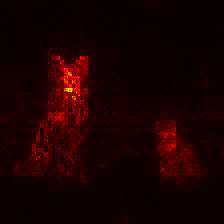
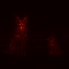
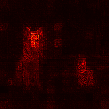
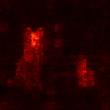
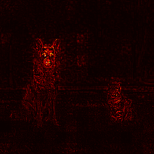
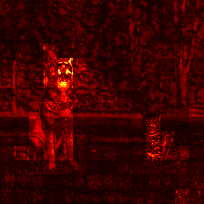
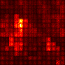
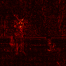
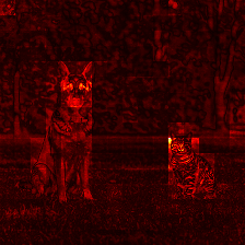
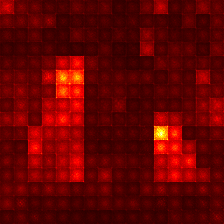
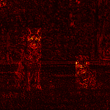
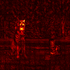
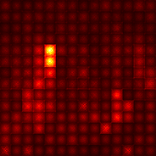
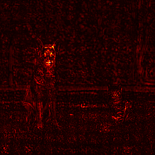
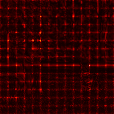

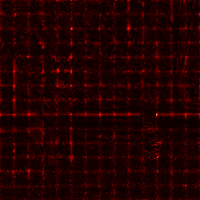
Look closely at the full-resolution maps and the patch grid bleeds through. WSquare outlines the patch borders sharply, $z^+$ softens them, and Gamma erases them almost completely. The number under each map measures this as the contrast between neighbouring pixels across a patch border compared with inside a patch, where 1 means no edges. Over the five images, the median for ConvNeXt is 2.11 with WSquare, 1.66 with $z^+$, and 0.97 with Gamma, and Swin and the DINO ViTs behave the same way.
MAE is the exception. Its grid survives all three rules, and Gamma leaves it almost as strong as $z^+$ does. Its first layer looks unusual too, putting more than half of its squared weights on the outermost pixels of each patch. These pixels make up less than a quarter of a patch, and in DINOv1 and the supervised ViT they receive a share in line with their number. Even the plain gradient shows the same grid, so it is not an artefact of LRP.
All rules at a glance
The table below lists the rules chosen early on, WSquare for ConvNeXt, Swin, and MaxViT and $z^+$ for the ViTs. By these numbers, Gamma would be the better choice for all of them except MAE, where no rule removes the grid.
| ResNets | ConvNeXt | Swin | MaxViT | Plain ViTs | |
|---|---|---|---|---|---|
| first layer | $z^+$ | WSquare | WSquare | WSquare | $z^+$ |
| layers inside blocks | $z^+$ | Gamma | Gamma | Gamma | Gamma |
| activations, layer scale, gates | pass | pass | pass | pass | pass |
| LayerNorm | — | spread constant | spread constant | spread constant | spread constant |
| attention | — | — | weights constant | weights constant | weights constant |
| residual split | equal | proportional | proportional | magnitude | magnitude |
Conclusion
Maps like these do more than catch shortcuts like the horse copyright tag at the start. They can also point to quirks of the architecture itself. The checkerboard in ResNet-50 traces back to how its strided layers are wired, and ResNet-D, a later variant, removes the same weakness by averaging before the shortcut [He et al.].
MAE’s maps stay nearly flat and carry a grid along its patch borders that no first-layer rule removes. To the eye, the result looks uninformative, with almost no visible object outline. Still, the underlying relevance may carry semantic signal concentrated along those patch edges rather than across object interiors, as the interactive visualization suggests, though confirming this quantitatively remains an open question.
Ultimately, LRP is only as trustworthy as the rules defined for the architecture underneath it, with conservation offering a built-in sanity check. Once every block has a proper rule, LRP remains a practical way to expose data shortcuts and architectural weaknesses in modern vision models, even without labels.