
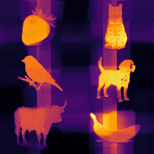
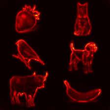
Foundation models trained without explicit labels can learn remarkably rich representations, but the same lack of supervision that makes this possible also makes them harder to interpret and validate. Without annotations to tell us what the model has learned, where can we look for clues? Convolutional networks and vision transformers offer one in their activations. These activations can be turned into heatmaps that show where the model responds most strongly, without extra labels or gradients. The catch is that these maps are often coarse. In this blog post, we explore how to extract spatial heatmaps from these activations and how they can be refined.
This journey started with my attempt to use generative adversarial networks (GANs) as feature extractors for medical images. GANs can synthesize high-quality images from random noise and provide control over the generation via latent variables, but they are not inherently invertible. I tried to address this limitation, but the approach did not work well (see my earlier post for details). Debugging that encoder-based GAN quickly became an exercise in frustration. More importantly, it exposed how few tools exist for debugging models trained without explicit annotations. The limitation is particularly relevant in self-supervised learning (SSL), where useful representations are learned directly from unlabeled data. This gap motivated me to investigate ways of deriving attribution maps for models trained without explicit labels. As part of this investigation, I found that simply averaging the feature activations produces surprisingly coherent spatial maps [Karjauv et al.].
All figures and numbers in this post can be reproduced with the companion notebook, which also contains the code for the maps and for LRP, as well as small step-by-step implementations of RISE, RELAX, CAM and Grad-CAM.
Self-Supervised Learning Meets XAI
Learning without labels matters because collecting data is often much easier than annotating it, especially at scale. SSL makes it possible to use that unlabeled data to learn representations that can later be reused or fine-tuned for downstream tasks, such as image classification or segmentation. At the core of these models is an encoder, a network that turns an input image into a compact set of features called an embedding. In a supervised classifier, this embedding is typically passed to a prediction head that produces class scores. SSL models such as SimCLR and DINO instead train the encoder on a proxy task, such as matching different augmented views of the same image. The proxy task is only a means to learn good features. Once training is done, it is discarded, and what remains is an encoder with no task of its own. At sufficiently large scale, models trained this way can also form the basis of foundation models.
The absence of labels, however, also makes it difficult to verify whether the learned representations are actually relevant for a given downstream task. For example, a model trained on images of cars may learn features related to wheels, windows, and overall vehicle shape. Some of these features may transfer well to other types of vehicles, while others may be of little use when the model is applied to bicycles or motorcycles. Without labels, it is difficult to know which properties the model has learned and how useful they will be beyond the training data. Moreover, training on random crops can lead a model to memorize unintended associations, such as which object belongs in front of a particular background. Such associations can easily go unnoticed, and evaluating them is non-trivial [Meehan et al.].
This is where explainable AI (XAI) would seem useful. For supervised models, methods such as Grad-CAM can highlight image regions that contribute to a particular prediction. Occlusion methods such as RISE take a different route. They repeatedly mask parts of the input and observe how the target prediction score changes.
For an SSL encoder, however, there may be no prediction score to explain. The model produces an embedding, and its individual dimensions usually have no predefined semantic meaning. We do not know that one feature represents a wheel, another a window, or another the shape of a car. Asking for the importance of a pixel for the class “car” therefore makes little sense when there is no car score in the first place.
There have been attempts to adapt XAI to label-free models. One such attempt is RELAX (Representation Learning Explainability), which extends the supervised occlusion method RISE. Instead of asking how masking part of an image changes a class score, we can ask how much the masking changes the representation. The original image provides a reference embedding. Masked versions of the image are passed through the same encoder, and their embeddings are compared with the reference using cosine similarity. If masking a region substantially changes the representation, that region was probably important to the encoder.
The idea is simple, but it comes at a cost. RELAX requires many masked versions of each image and therefore many forward passes through the model, while the resulting maps can be noisy. More generally, masking itself is not entirely innocent. Hiding parts of an image with a solid color creates inputs that differ from what the model normally sees, so part of the response may come from the perturbation.
From Class-Specific to Label-Free Activation Maps (LaFAM)
One useful property of CNNs is that their convolutional feature maps retain a spatial layout. If a feature responds strongly in one part of the image, we can trace that response back to roughly the same region in the input. This spatial structure is what makes methods such as class activation maps (CAMs) possible.
What are activation maps and receptive fields?
Each convolutional layer produces a collection of activation maps (also called feature maps), one per feature channel. Each map records how strongly a learned feature responds at different spatial locations. Together, these maps form a feature tensor. Early layers often respond to relatively simple patterns such as edges or color contrasts. Deeper layers combine these responses into more complex representations. These can become selective to textures, shapes, object parts, or other structures useful to the model, although individual channels do not necessarily correspond to clean human-interpretable concepts.
Each activation is influenced by a region of the original image called its receptive field. Receptive fields grow as convolutional layers are stacked. Pooling and strided convolutions increase them further while reducing spatial resolution. As a result, deeper feature maps capture information from larger regions of the image but provide a progressively coarser spatial view.
In the original CAM formulation, the classifier assigns a different weight to each feature channel for each class. To explain a prediction such as car, CAM reduces the stack of spatial activation maps to a single heatmap using the weights associated with the car class. Features that are strongly associated with that class contribute more to the resulting heatmap. Grad-CAM generalizes this idea by using gradients to estimate how important each feature map is for a chosen target. In other words, the activation maps tell us where a feature responds, while the class-specific weights tell us which features matter for the target.
But what if there is no class to explain? We can take a surprisingly simple approach. Instead of finding class-specific weights, we give every feature channel equal weight and average the activations across channels at each spatial location. In the ResNet-50 models evaluated in the LaFAM paper, the final activations come out of a ReLU, which sets negative responses to zero. Positive and negative values therefore cannot cancel when averaged. A location receives a high value when many high-level features respond there, or when a smaller number respond particularly strongly. While CAM asks the classifier which feature maps matter and then combines them accordingly, averaging simply lets every feature map vote equally.
What About Vision Transformers?
ViTs come with a tempting visualization: attention. We can inspect how image patches attend to one another and map those interactions back onto the image. In self-supervised models such as DINO, attention maps can even reveal surprisingly clear object structure without segmentation labels. But attention tells us how tokens exchange information, not necessarily which parts of the image are responsible for the representation we want to inspect. So what happens if we leave attention aside and look at the token representations themselves?
A ViT divides an image into patches and represents each patch with a token. The tokens are processed as a sequence and exchange information through self-attention, so a token in a deep layer no longer describes only its own patch. Still, every patch token has a known spatial address in the original image, which means we can arrange them back into their original grid. Many ViTs, such as the supervised ViT and CLIP, are trained through an extra class token, and only that token reaches the classifier. Even so, the patch tokens preserve where things are in the image [Raghu et al.], and we can read this information from them. This gives us something similar to a CNN feature tensor. In a CNN, each spatial location contains a vector of channel activations. In a ViT, each patch contains a token vector, and we call its entries channels as well. Reduce each token to a single value, put the values back into the patch grid, and we get a coarse heatmap.
The reduction itself requires a choice. Unlike the ReLU outputs of a ResNet, ViT tokens are signed, and so are the features of modern CNNs such as ConvNeXt. Individual channels also have no predefined semantic meaning. Different features may respond to objects, object parts, textures, or surrounding context. Collapsing them into a single value therefore produces a summary of where the representation is active. Here, we apply ReLU before averaging, which keeps the positive responses and prevents them from cancelling against negative ones. We use this same reduction for every model below, so the maps show where positive feature responses are strongest. It is not the only reasonable choice, and it does not work equally well for every encoder, as we will see further below.
Results
ConvNeXt Base · Averaging

Dog and cat

Two dogs

Fish and person


Spider web

Six objects
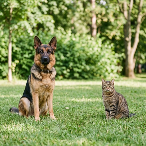
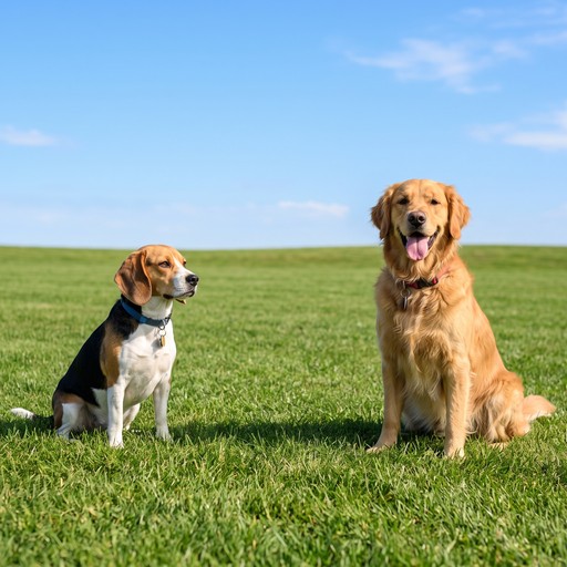
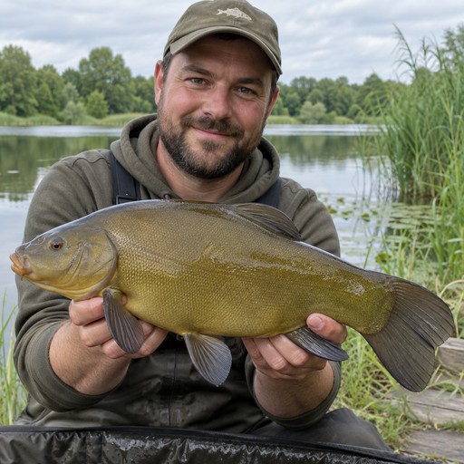
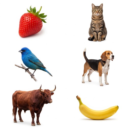
The grid shows label-free heatmaps from a supervised ConvNeXt for five images, four of which contain several objects. When a scene contains more than one object, the map does not pick a winner. The dog and the cat both light up, and so do both dogs and all six objects. With no class to choose, every object the encoder responds to strongly stays in the map.
The limitation is just as easy to see. ConvNeXt, like ResNet-50, ends with a $7\times7$ grid of features. The response is already informative, but it is coarse. Nearest-neighbor resizing shows it as large tiles, and bilinear resizing would only blend their edges.
Supporting evidence: the evaluation in the LaFAM paper
The paper systematically compares averaging with RELAX (the prior SSL method) using SSL models (SimCLR and SwAV with ResNet-50 backbones). It also compares averaging with Grad-CAM for a fully supervised ResNet-50 classifier as a sanity check. The heatmaps for ResNet-50 are only $7\times7$ and were upscaled to the input image size with nearest-neighbor interpolation. Since we don’t have class labels to evaluate the “correctness” of an explanation, the evaluation was performed on datasets with segmentation masks (ImageNet-S and PASCAL VOC), using a suite of metrics from the Quantus XAI evaluation framework. Essentially, we treat it as a localization task, with the goal of assessing how well the heatmaps align with the segmentation masks.
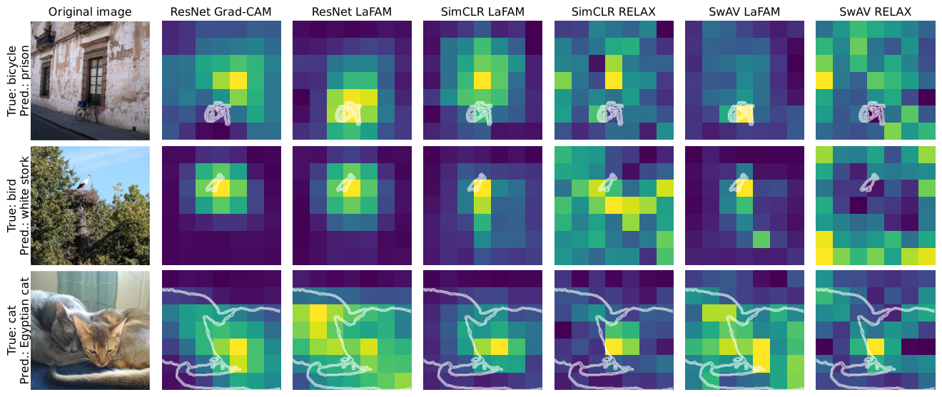
The figure above compares averaging, RELAX, and Grad-CAM as a baseline. When applied to the same supervised model, averaging and Grad-CAM produce very similar heatmaps.
In the first row, the model predicted the wrong ImageNet class, so Grad-CAM highlighted a region associated with that wrong class. Averaging does not depend on the predicted label, so it still shows what the model found salient. For SSL models, averaging produces notably less noisy heatmaps than RELAX.
The next figure demonstrates that averaging, being class-agnostic, highlights multiple objects in the image (e.g., both dogs), whereas Grad-CAM focuses on the one tied to the predicted class.
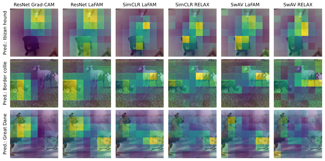
The last figure shows more misclassified ImageNet examples, with Grad-CAM computed for the wrong predicted class.
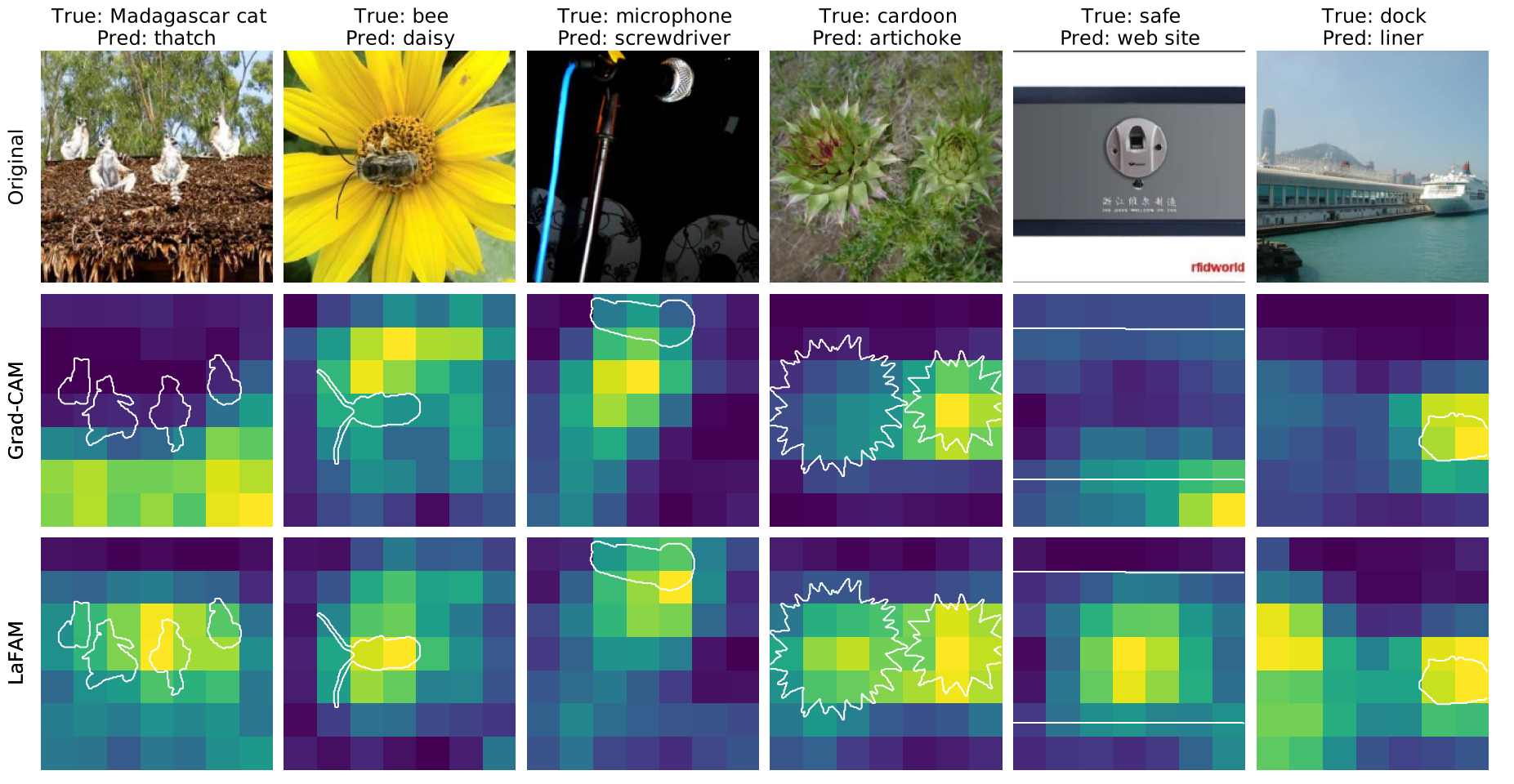
The averaged heatmaps clearly highlight true objects, suggesting that these objects strongly activate multiple channels in the final convolutional layer. However, the prediction is wrong. The reason could be that the last fully connected layer puts more weight on specific features that mislead the final decision, even though many other features correctly identify the object.
| Metric | Supervised (ResNet-50) | SSL (SimCLR) | SSL (SwAV) | |||
|---|---|---|---|---|---|---|
| Grad-CAM | LaFAM | RELAX | LaFAM | RELAX | LaFAM | |
| Pointing Game | 94.00 | 90.67 | 88.29 | 92.14 | 85.47 | 89.90 |
| Sparseness | 42.74 | 34.82 | 35.26 | 49.70 | 31.49 | 39.92 |
| Relevance Mass Accuracy | 50.28 | 45.89 | 46.19 | 53.32 | 42.96 | 50.13 |
| Relevance Rank Accuracy | 62.22 | 59.50 | 58.13 | 61.44 | 53.64 | 64.69 |
| Top-K Intersection | 75.07 | 69.09 | 71.21 | 76.59 | 63.83 | 71.68 |
| AUC | 83.12 | 80.45 | 76.49 | 81.28 | 70.13 | 83.03 |
| Metric | Supervised (ResNet-50) | SSL (SimCLR) | SSL (SwAV) | |||
|---|---|---|---|---|---|---|
| Grad-CAM | LaFAM | RELAX | LaFAM | RELAX | LaFAM | |
| Pointing Game | 90.83 | 91.23 | 91.63 | 94.68 | 82.73 | 93.62 |
| Sparseness | 44.39 | 36.20 | 36.04 | 51.00 | 32.36 | 41.61 |
| Relevance Mass Accuracy | 40.44 | 37.13 | 38.00 | 45.67 | 34.18 | 42.17 |
| Relevance Rank Accuracy | 53.53 | 53.94 | 54.55 | 58.73 | 46.40 | 61.05 |
| Top-K Intersection | 65.46 | 63.42 | 67.82 | 75.05 | 56.22 | 67.63 |
| AUC | 82.87 | 84.00 | 79.88 | 85.33 | 71.24 | 87.74 |
Pointing Game: Percentage of samples where the single most salient pixel falls inside the ground-truth object region.
Top-$K$ Intersection: Fraction of the top $K\%$ most salient pixels that lie within the true object region.
Relevance Mass Accuracy / Rank Accuracy: Metrics that assess how much of the total saliency "mass" falls within the object mask, or how well the saliency values are ordered (foreground > background).
Sparseness: A measure of how concentrated the heatmap is. Higher means the map is tight and focused; lower means it is more diffuse or noisy.
AUC (Area Under the Curve): Treats every pixel’s saliency value as a prediction of “foreground vs. background” and measures how well these values separate the two groups. A high AUC means the object pixels generally have higher values than background pixels.
These measurements show that channel-averaged feature activity can localize annotated objects in the evaluated CNNs, including the self-supervised models. They do not establish that every active feature is an object detector or that the network has discarded all background information. Nor does a bright region under a wrong prediction prove that the model recognized the object correctly.
The metric choices also matter. Sparseness is not a measure of correctness. The localization metrics do use annotations and can penalize responses to real but unannotated objects. This becomes especially important when we compare methods that produce very different amounts of fine detail, as we will see below.
A Finer Picture
The coarse grid comes from the encoder itself. CNNs progressively downsample the image, and ViTs cut it into fixed-size patches. To obtain a finer map, we can either upsample the features with AnyUp or propagate the activations back to the input using LRP. Both approaches increase spatial detail, but they do so in very different ways.
AnyUp [Wimmer et al.] is a pretrained feature upsampler designed to work with features from different vision encoders. It takes low-resolution features together with the corresponding higher-resolution image and upsamples the feature tensor to the image resolution. During training, the encoder’s features for a small crop serve as a finer-scale target for the same region of the full image, so AnyUp learns to predict what the features would look like at a higher resolution. The image provides spatial guidance that ordinary interpolation does not have.
For example, ConvNeXt turns a $224\times224$ image into a $1024\times7\times7$ feature tensor. We can give AnyUp this tensor together with the image, and it produces a $1024\times224\times224$ feature tensor. We can average its channels in the same way as before to obtain a full-resolution heatmap. Under the hood, every output feature vector is a weighted average of the coarse feature vectors in a small window around it, with the weights computed by attention between the image pixels and the coarse features. When the features are already non-negative, as in a ResNet, the same holds for the heatmap, since averaging over channels is linear as well. Each pixel of the refined map is then a weighted average of nearby cells of the coarse map. AnyUp decides where the boundaries between them run, but it cannot create a response the coarse map does not have.
Layer-wise relevance propagation (LRP) [Bach et al., Montavon et al.] takes a different approach. Instead of increasing the resolution of the feature tensor, it traces relevance backward through the encoder. At each layer, relevance is redistributed to the preceding neurons according to a chosen propagation rule until it reaches the input, producing a pixel-level attribution map. It was originally designed to explain predictions from supervised models by redistributing the relevance of a target output back to the input. But nothing prevents us from choosing a different starting signal. Instead of a class score, we start from the encoder’s features themselves. We place a fixed amount of relevance on the feature tensor and let LRP carry it back to the pixels. Each feature value receives a share in proportion to how strongly it is active, so inactive features start with nothing. This is the same quantity the averaged map shows, the positive feature activity, now traced back to the input. The resulting map shows which input pixels the propagation connects to the active features at the chosen layer.
The figure below shows the CNNs, two transformers that restrict most of their attention to local windows, and three plain vision transformers. Three more plain ViTs follow in a separate figure further down, because the same reduction fails for them.
Real images · compare encoder responses
Two dogs1 / 5
How to use this figure
Pick an image from the dock, then read across a row to compare the coarse heatmap produced by averaging with its AnyUp refinement and with the relevance LRP propagates back to the pixels. Move over a map and it falls away around the pointer; press and hold to clear the whole map from the point you pressed, and let go to bring it back. On a touch screen, tap a map or hold a finger on it.

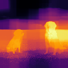
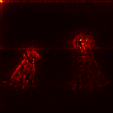
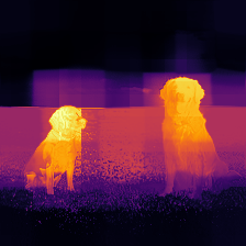
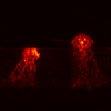

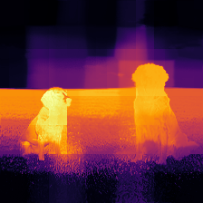
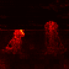

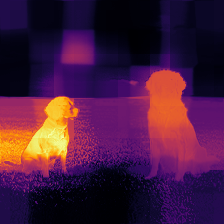
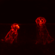

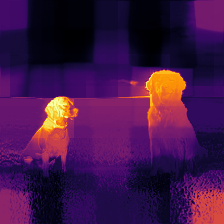
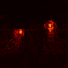

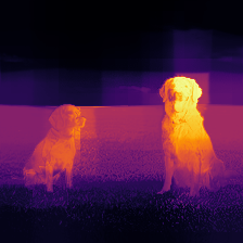
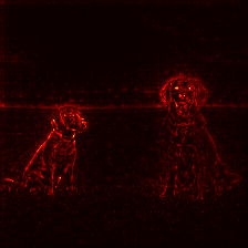

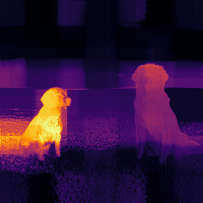
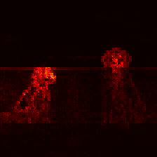

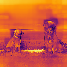
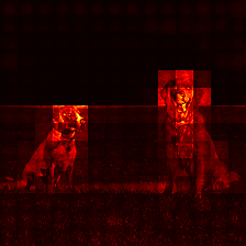

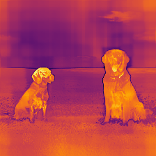
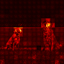

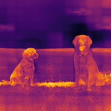
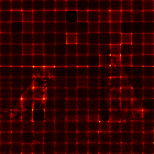
The Averaging column is blocky by construction, since each block is one feature cell. An object shows up as a cluster of bright blocks that spills over its edges into the background. AnyUp keeps that pattern but redraws it to follow the image. The blocks around the two dogs become two dog silhouettes, and the cluster over the fish takes on the fish’s outline. Each object comes out filled in almost evenly, with a sharp border wherever the image has one.
The glow that spills into the background can come from three places. At $7\times7$, a cell on the edge of an object covers part of the object and part of the background. Each cell also sees more of the image than its own square. In a CNN, each feature is computed from a wider region around it, and in a transformer, attention lets each token gather information from other tokens. A patch of grass next to a dog can therefore carry information about the dog. Finally, the background can matter in its own right. Grass, trees, and sky are things an SSL model can learn to recognize, just like dogs. The background may also serve as a shortcut, as when a model learns to expect a dog wherever it sees a lawn. AnyUp cannot tell these cases apart. Each refined value is a weighted average of nearby coarse values, so AnyUp keeps whatever the coarse map contains and only gives it sharper edges.
LRP shows a different picture. Its relevance concentrates on image structures such as contours, object parts, and internal edges, and little of it reaches the background. The maps are sparse, and they are not free of artifacts either. The CNN attribution maps are generally spatially continuous, whereas Swin shows visible block structure in some of the images. The plain ViTs show blocks the size of their patches, and for MAE a regular grid dominates much of the relevance map. Producing a pixel-level attribution map therefore does not remove the spatial constraints introduced by patch embeddings or by the chosen propagation rules.
One caveat is that the Zennit library I used provides built-in support mainly for VGG and ResNet architectures. ConvNeXt and ViTs contain operations for which I had to implement additional propagation rules, as others have done for transformers [Achtibat et al.]. These LRP attribution maps should therefore be read as the result of one reasonable set of propagation choices. I will go through these choices, and how much they change the maps, in an upcoming post.
A note on evaluation
The original LaFAM paper evaluated attribution largely as an object-localization problem, using segmentation masks as ground truth. This works reasonably well for comparing coarse maps, but becomes harder to interpret once the maps contain fine spatial structure. Mask-based localization treats the annotated object region as the target, without distinguishing which parts of that object actually contributed to the representation. A fine-grained map of a bicycle, for example, might concentrate on its frame, wheels, or other structures, while a smoother map spreads its response across much of the object. Some localization metrics can favor the latter because more of the annotated region receives high attribution, even though the map contains less spatial detail. Thin structures may also be imperfectly represented in the segmentation mask itself. Label-free maps introduce another mismatch: responses to other objects are counted as background even when the encoder genuinely responds to them.
A Watermark in the Web
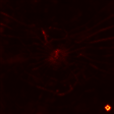
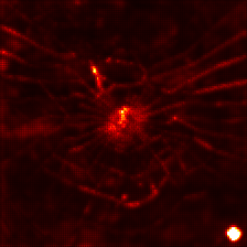
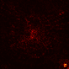
The spider web image holds a small surprise. In its bottom-right corner sits a tiny sparkle, the watermark of the image generator that created the picture. It covers less than one percent of the image and is easy to miss, but several encoders do not miss it. This is the kind of finding that makes label-free maps useful for debugging. Nobody asked the models about the watermark, and no label points to it, yet the maps show that the models respond to it.
The two methods reveal it in different ways. For CLIP ConvNeXt, the watermark’s cell is the brightest of all 49 cells in the averaged map, and LRP places about five percent of the relevance on it. MaxViT barely reacts to the watermark in the averaged map, but its LRP map puts almost eight percent of the relevance there, with a peak about four times higher than anywhere else. Since every map is scaled by its own maximum, that single spot turns the rest of the MaxViT map nearly black.
Spider web · a watermark in the corner

MaxViT · Averaging
MaxViT · LRP
MaxViT · LRP, scaled without the watermark

CLIP ConvNeXt · Averaging
CLIP ConvNeXt · LRP
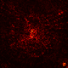
CLIP ConvNeXt · LRP without the watermark cell
Once we know about the watermark, we can set it aside and look at the rest. For CLIP ConvNeXt, it is enough to leave the watermark’s cell out of LRP’s starting amount. The share on the watermark then drops from five to about two percent, and the center of the web becomes visible, although the map stays noisy. For MaxViT, the same step changes almost nothing, because relevance reaches the watermark from cells across the whole image, even from the opposite corner. Only when the map is scaled without the watermark does it become clear that the threads of the web were there all along.
The example also shows where the maps stop. They tell us where the representation responds, but not what the response is about. We recognized the watermark because we looked at the image ourselves. To the maps, it is just another bright region, like the web. Telling such responses apart without labels requires asking the representation something else, for instance which parts of an image it treats as alike. Why a small watermark draws so much of the response is a question of its own, which we leave for a later post.
When ReLU Is Not Enough
The first figure includes three plain vision transformers, DINOv1, DINOv3 and MAE, and their maps behave much like those of the CNNs. For three other plain ViTs, a supervised ViT-B/16, a CLIP ViT-B/16 and DINOv2, the same reduction fails. Their maps are bright almost everywhere apart from a handful of much darker tokens, and the objects are hard to find.
Real images · plain vision transformers
Dog and cat1 / 5
How to use this figure
Pick an image from the dock, then read across a row. The first map applies a ReLU and averages over the channels, as in the gallery above. The second first subtracts each channel's average over the image. The third refines the centered map with AnyUp, and the fourth shows LRP. Move over a map and it falls away around the pointer; press and hold to clear the whole map, and let go to bring it back.


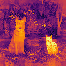
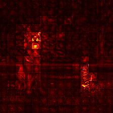


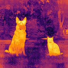
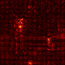


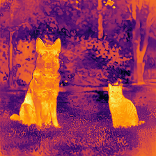
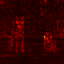
What sets the two groups apart? The obvious suspect is the ReLU, but it does not throw most of the values away. In every plain ViT we looked at, about half of all feature values are positive, just as in the CNNs. Two other differences stand out.
The first is the dark tokens. All three encoders that fail have some of them in the background of every image, while DINOv1, DINOv3 and MAE have none. Such outlier tokens are a known effect in ViTs [Darcet et al., Sun et al.]. Darcet et al. found them in DINOv2, a supervised ViT and OpenCLIP, but not in the original DINO. They also showed that a few extra tokens, called registers, remove them, and DINOv3 has four such registers. A heatmap is stretched between its darkest and its brightest token, so these few dark tokens use up most of the color scale, and nearly all other tokens end up bright.
The second is the channels that never switch off. In a CNN, a channel is usually active in some parts of the image and inactive in others. In a ResNet, inactive means zero, and in ConvNeXt it means negative. In the supervised ViT and CLIP, between one channel in eight and one in six stays positive across almost the whole image, and these channels are strongest on the background. The ReLU passes them unchanged, so they pull the map away from the objects. The other plain ViTs have such channels too, but too few or too weak to shape the map. For the supervised ViT, leaving out these channels and setting the color scale without the outlier tokens is enough to bring the objects back.
The remedy is to center each channel before the ReLU. From every channel, we subtract its average over all tokens of the image. The channel is then positive exactly where it is higher than usual in this image, whatever its overall level. Like the plain average, this needs no labels, no other images and no backpropagation.
For the three encoders that failed, centering helps, but the maps stay far from clean. Only the image of the dog and the cat and the image with six objects come out readable. In the image of the dog and the cat, both animals stand out for CLIP and DINOv2, while the supervised ViT shows the cat clearly and the dog only faintly. The other images stay noisy. The remaining encoders work without centering, which is why the first figure keeps the original reduction for all of them.
In the photo of the fish, the supervised ViT shows the fish darker than the person holding it. The classifiers may not need the fish much. If we remove it from the photo, every classifier in this post still predicts a tench. ImageNet photos of tench usually show an angler holding the catch, so the models have learned the scene rather than the fish. This is a known shortcut [Geirhos et al.], and finding such shortcuts is exactly what attribution methods were designed for.
A closer look at the channels and the outlier tokens
A channel counts as never switching off here if it is positive at nine out of ten tokens of an image or more. All six plain ViTs have such channels, but only in the supervised ViT and CLIP are they numerous enough to shape the map.
Why ViTs have such channels, we can only guess. A ResNet applies a ReLU itself, so zero is a meaningful dividing line for its features. A ViT does not, and for many of its channels zero seems to be an arbitrary point. ConvNeXt has no ReLU at its output either, but its channels cross zero within an image, which fits with its maps working without centering.
Centering only shifts the channels and does not rescale them. Dividing each channel by its spread as well gave almost the same results in our tests, so the shift is what matters.
The outlier tokens are a separate problem. Setting the color scale without them brings back the contrast, but not clear objects. They are also not weak inside the network. Just before the output, each of them has one channel with an enormous value, the same channel in every image. In the supervised ViT, this value reaches about a thousand, while the largest value of an ordinary token is a few dozen.
The last step of these encoders is a layer normalization. It divides each token by the spread of its values, so that all tokens end up on a similar scale. In an outlier token, that spread comes almost entirely from the one huge channel. Dividing by it leaves the spike as the only large value and pushes all other channels close to zero. The token becomes nearly flat. The ReLU map counts only values above zero, and a flat token has very little of them, so it comes out darkest.
Centering compares each channel with its own average in the image instead of with zero. In the supervised ViT, about a third of the channels are clearly negative on average over the image. For them, a value near zero is well above average. A flat token therefore scores high in all these channels at once, and some of the outlier tokens become bright spots in the centered maps. DINOv2 has fewer such channels, and its outlier tokens stay dark. In neither map does their brightness tell us anything about the image at their position. Only the reference they are compared with has changed.
AnyUp works well on the centered features. It turns the token grid into object silhouettes, much as it does for the CNNs, and its maps show the objects at least as clearly as the centered maps they come from. LRP starts from the same positive activity as the plain average, yet for these three encoders its maps still show the objects, with the same patch-sized blocks as the other plain ViTs.
Limitations
Resolution. The heatmap produced by averaging can only be as sharp as the feature grid being averaged, namely $7\times7$ for the CNNs here and $14\times14$ for ViT-B/16. On a $224\times224$ input, one cell of a $7\times7$ grid spans $32\times32$ pixels. Small objects may disappear into a single cell, and nearby objects may merge into one response. Both refinements add detail, but each brings its own assumptions.
-
AnyUp takes its detail from the image. Its authors model each refined feature as a weighted average of nearby coarse features, a simplification they acknowledge themselves. The image decides the weights and aligns coarse responses with sharp image boundaries, but it cannot tell whether those boundaries reflect evidence the encoder used, so a background response can look just as precise as an object.
-
LRP takes its detail from the network’s own computation, but the result depends on where relevance starts and which propagation rules carry it. LRP deliberately allows different rules, and its authors leave the choice to the particular model, problem, or practical requirements instead of prescribing a general procedure. These choices can visibly change the maps.
What does the heatmap mean? Averaging collapses the feature dimension into a single value at each spatial location. This gives us a useful spatial summary, but it throws away information about which features produced the response. Two bright regions may be driven by entirely different features, and the map cannot tell an object from a background texture if both produce strong activations. This is particularly important for self-supervised models, where the individual feature dimensions have no predefined semantic meaning.
The reduction itself is also a choice. Here, we apply ReLU before averaging, so negative values are discarded, and as we saw above, this breaks down for some encoders unless each channel is centered first. We could instead average the signed values directly, average their absolute magnitudes, or summarize each feature vector by its norm. These operations emphasize different properties of the representation and need not produce the same heatmap. Why such simple summaries preserve coherent spatial structure at all is therefore not obvious.
Finally, a strong response does not tell us whether that response matters for a particular task. The averaging procedure has no prediction target, so a bright region may contain useful object information, contextual information, or a feature that a downstream classifier never uses. The map tells us where the representation responds, but not what the response represents or what it will ultimately be used for.
Conclusion
Averaging across feature channels is almost embarrassingly simple. It ignores what the individual features mean, gives them all the same weight, and does not ask the model for a prediction. Yet the resulting maps repeatedly line up with coherent objects and other structures in the image.
Look back at the scenes with several objects, though. Supervised models trained with one label per image must name a single class. Yet their maps highlight the dog and the cat, both dogs, and all six objects. So what happens to everything they see but never name?
The answer points to something deeper than our starting question, namely that models see far more than we ever asked them to. In my recent work [Karjauv], I demonstrate that this is no accident. Classifiers with global average pooling and a linear head decompose cleanly into spatial evidence. Beneath the final prediction, the network quietly behaves like a multi-instance learner.
Then there is the background. If every location carries evidence, what makes the models respond strongly to objects, while “irrelevant” regions stay quiet?
SSL models never even get that one label. So when their maps light up, what exactly are they responding to, and how would we know?
Those are the questions I will turn to next.