Turning StyleGAN into a latent feature extractor

While Generative Adversarial Networks (GANs) are primarily known for their ability to generate high-quality synthetic images, their main task is to learn a latent feature representation of real data. In addition, recent improvements to the original GAN allow it to learn a disentangled latent representation, enabling us to obtain semantically meaningful embeddings.

This property could possibly allow GANs to be used as high-level feature extractors. However, the problem is that the original GAN architecture is not invertible or, in other words, it is impossible to project real images into the latent space. This article addresses this issue and attempts to answer whether GANs can extract meaningful features from real images and if they are suitable for downstream tasks.

StyleGAN [1] has revolutionized the creation of synthetic images and its successor, StyleGAN2 [2], has become the de-facto base for many state-of-the-art generative models. One of the reasons for this is that, along with high quality, it attempts to solve the problem of latent space entanglement and thereby makes each latent variable control a single abstract function by introducing perceptual path length (PPL) regularization.

Disentangled representations are a type of representation in which the factors of variation in the data are represented in a separate and independent way in the representation. This means that each dimension of the representation corresponds to a single factor of variation, and changing that dimension only affects that factor and not any others (e.g., hairstyle for human faces).

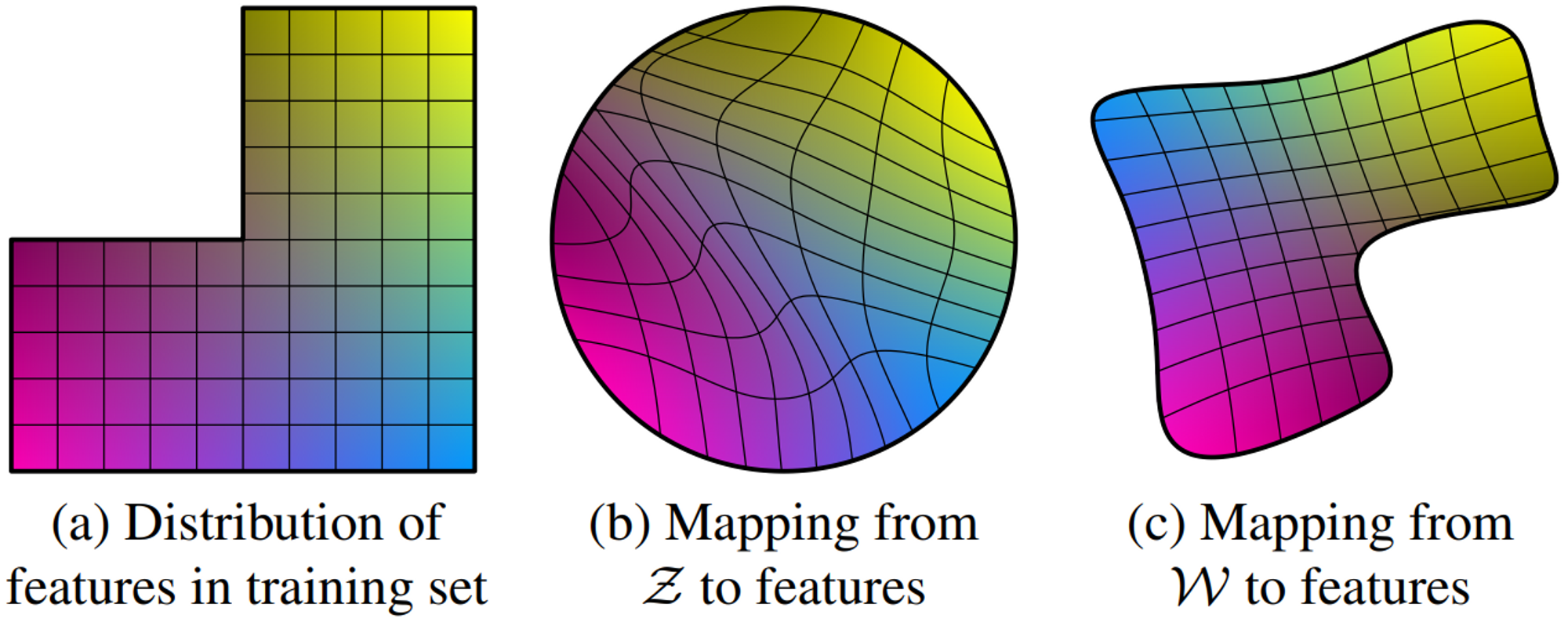
Illustrative example taken from StyleGAN [1]. Two factors of variation (image features, e.g., masculinity and hair length): (a) An example training set where some combination (e.g., long-haired males) is missing. (b) This forces the mapping from $\mathcal{Z}$ to image features to become curved so that the forbidden combination disappears in $\mathcal{Z}$ to prevent the sampling of invalid combinations. (c) The learned mapping from $\mathcal{Z}$ to $\mathcal{W}$ is able to “undo” much of the warping.

GAN can be viewed as a self-supervised representation learning approach with contrastive loss, where real images are positive examples and the generator produces negative ones.

As mentioned, one of the limitations is that a common GAN is non-invertible, meaning it can only generate images from random noise and cannot extract embeddings from real images. Although there are methods to project real images into GAN’s latent space, the most popular is slow and computationally expensive as it is based on an optimization approach. Instead, we can train an encoder along with the generator and discriminator.

As mentioned, one of the limitations is that a common GAN is non-invertible, meaning it can only generate images from random noise and cannot extract embeddings from real images. Although there are methods to project real images into GAN’s latent space, the most popular is slow and computationally expensive as it is based on an optimization approach.  Instead, we can train an encoder along with the generator and discriminator. From this point of view, GAN can be viewed as a self-supervised representation learning approach with contrastive loss, where real images are positive examples and the generator produces negative ones.

Essentially, the discriminator in GAN already has an encoding part, as it is nothing more than a simple CNN binary classification model and CNNs are known to be good at extracting features from images. As a matter of fact, we can logically decompose it into a CNN encoder network and a fully connected discriminator network. So, Instead of adding another network, we can reuse the discriminator’s weights, saving memory and computational resources.

Architecture of Adversarial Latent Autoencoder [3].

The approach described in this article is based on the architecture proposed in “Adversarial Latent Autoencoders” (ALAE) [3]. To make the latent spaces of the Mapping network $F$ and encoder $E$ consistent with each other, the authors add an additional term to the GAN loss:

\[L_{\text{consistency}} = E_{p(z)}\bigg [ ||F(z) - E \circ G \circ F(z) ||_2^2 \bigg ]\]

This term forces the encoder to produce the same latent vector from a synthetic image used to generate it. More precisely, we first generate an intermediate vector from noise, $w = F(z)$, then generate a synthetic image from it, $x^\prime = G(w)$, and encode it back into an intermediate vector, $w^{\prime} = E(x^\prime)$. Finally, we minimize the $L_2$ norm between these vectors, $|| w - w^\prime||_2^2$.

In contrast to autoencoders, where the loss calculates an error element-wise in pixel space, this loss operates in latent space. The pixel-wise $L_2$ norm loss is one of the reasons why autoencoders have not been as successful as GANs in generating diverse and high-quality images [4]. Its application in pixel space does not reflect human visual perception, since an image shift of even one pixel may cause a large pixel-wise error, while its representation in latent space would be barely changed. Therefore, the $L_2$ norm can be used more effectively by applying it to the latent space providing invariance, such as for translation.

Additionally, ALAE introduces an information flow between the generator and discriminator, which makes the model more complex but can improve convergence speed and image quality. In this example, I leave it out to keep everything simple.

Implementation

To demonstrate this approach I chose an unofficial StyleGAN2 PyTorch implementation.

The main change is the introduction of a new loss term which I called consistency loss:

z = torch.randn(args.batch, args.latent, device=device)
w_z = mapping(z)
fake_img, _ = generator([w_z])
w_e = encoder(fake_img)
consitency_loss = (w_z - w_e).pow(2).mean()

Basically, that’s all. We could use the original implementation of the discriminator and slightly change it to return intermediate results, right after the last convolutional layer. But I find it much cleaner to split the discriminator into two independent networks: Encoder and DiscriminatorMini.

Since the Generator in this implementation is combined with the mapping network, I also split it into 2 separate networks: Generator1 and MappingNetwork.

Evaluation

To quantitatively evaluate the encoder, I trained a base ResNet18 model on raw images and linear logistic regression along with SVM with linear kernel on embeddings (this was done only for MNIST and PCam datasets).

The expected result is that the embeddings will be linearly separable and the accuracy of the base models will be similar to that of linear models. This assumption is based on the use of PPL, which enforces a disentangled and linearly separable latent space.

Visual inspection still remains the standard evaluation approach, so I generated synthetical images to check if the model was not broken and also visualized embedding using UMAP to see if they form clusters.

Results

I trained this model on three different datasets: MNIST, CelebA + FFHQ, and PCam, and moved the training logic to the solver_mnist.py, solver_celeba.py, and solver_pcam.py, respectively. Each of the solvers has been slightly adjusted to match the dataset requirements. There is also a notebook with pretrained models where you can reproduce the results.

MNIST

Since the images in the MNIST dataset are only 28x28 pixels (were converted to 32x32x3) and the dataset itself is very simple, I first trained the model on it to test whether there are no bugs and the algorithm works as expected.

python3 solver_mnist.py --path path/to/save/dataset --size 128 --name <Project name> --run_name <experiment name> --batch 32 --iter 10000 --augment --wandb

Where --name and --run_name are used for wandb logging. The description of the parameters for each solver can be found in the help strings.

First I generate some random images to see if the changes didn’t break the model:

Next, I check if the encoder produces latent features from the same distribution as the generator by encoding real images from the test set (that the model hasn’t seen) and generating new ones from these embeddings:

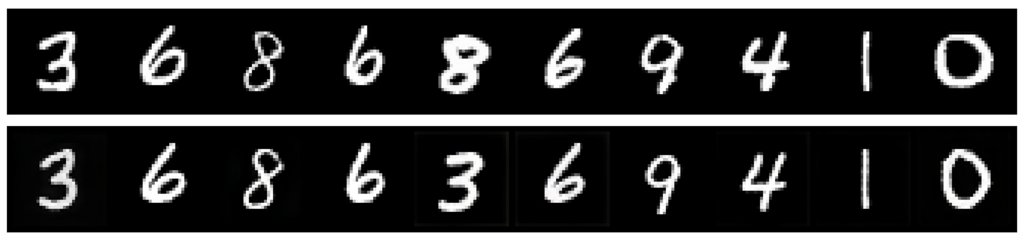
The first row represents the original images, the second row demonstrates the reconstruction

This figure demonstrates that the reconstruction works fairly well but is not ideal (one of the 8 was reconstructed into 3).

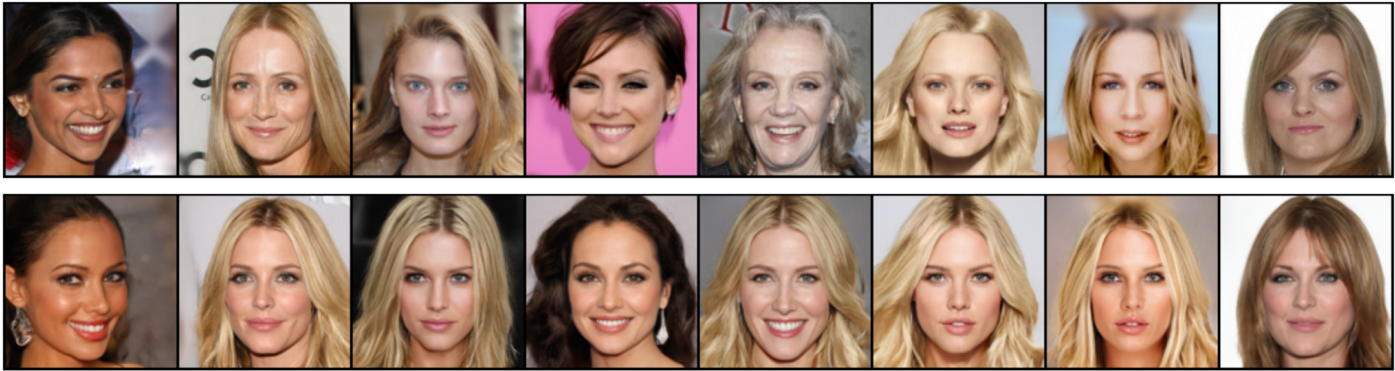
Additionally, I encoded the whole test set and used the embeddings to demonstrate querying top N similar images using cosine similarity:

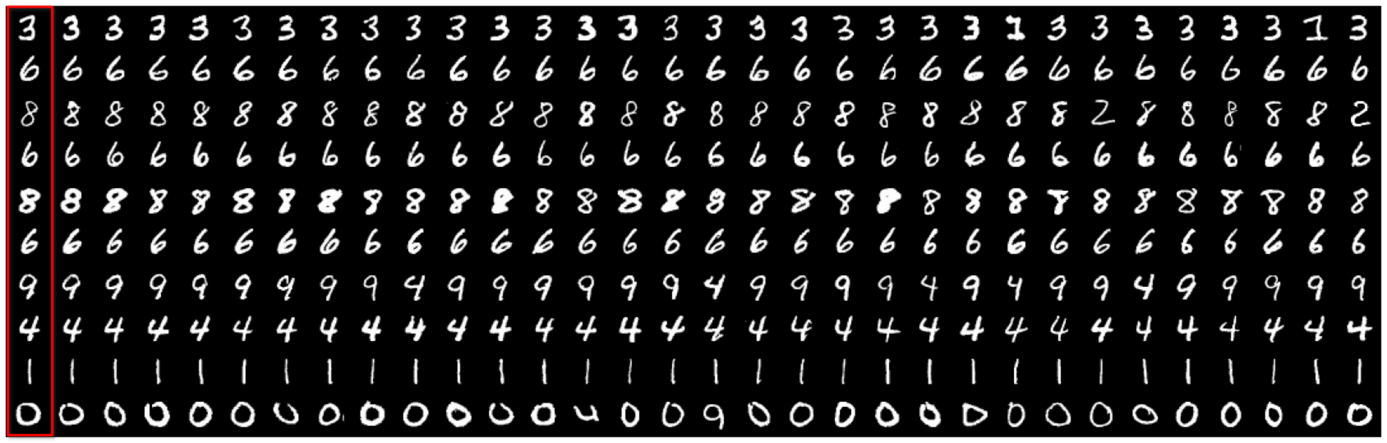
Searching for the most similar images. The first column contains real images

Now, we move on to quantitative assessment. As mentioned earlier, I trained linear SVM and logistic regression models to check if the embeddings are linearly separable. These models were trained on embeddings produced from half of the test set (which the GAN did not see) and the other half was used as a validation set. Both models reached 99% accuracy. The RestNet18 model was trained on the raw images from the training set and validated on the entire test set. It also achieved 99% accuracy which indicates that the GAN model has successfully learned the disentangled latent representation.

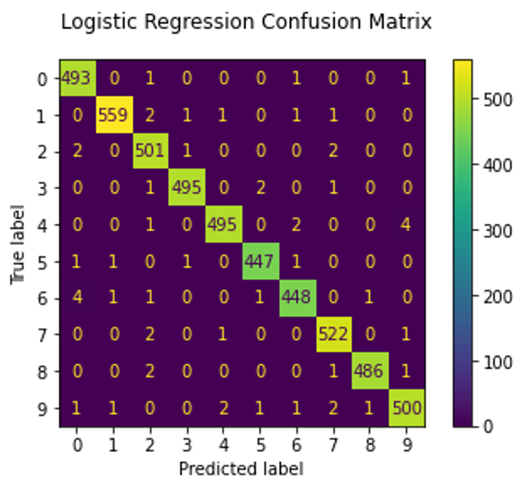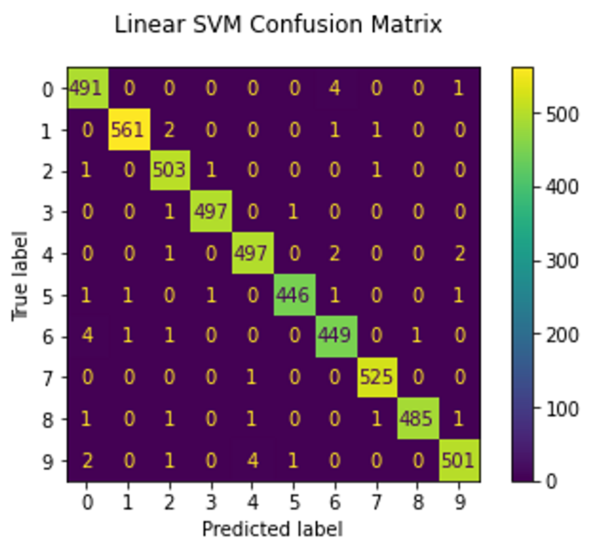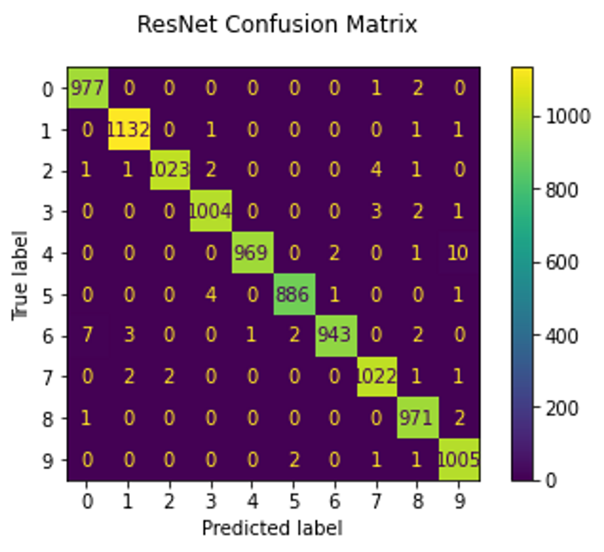Finally, I visualize the embeddings by projecting them into 2d space using UMAP:

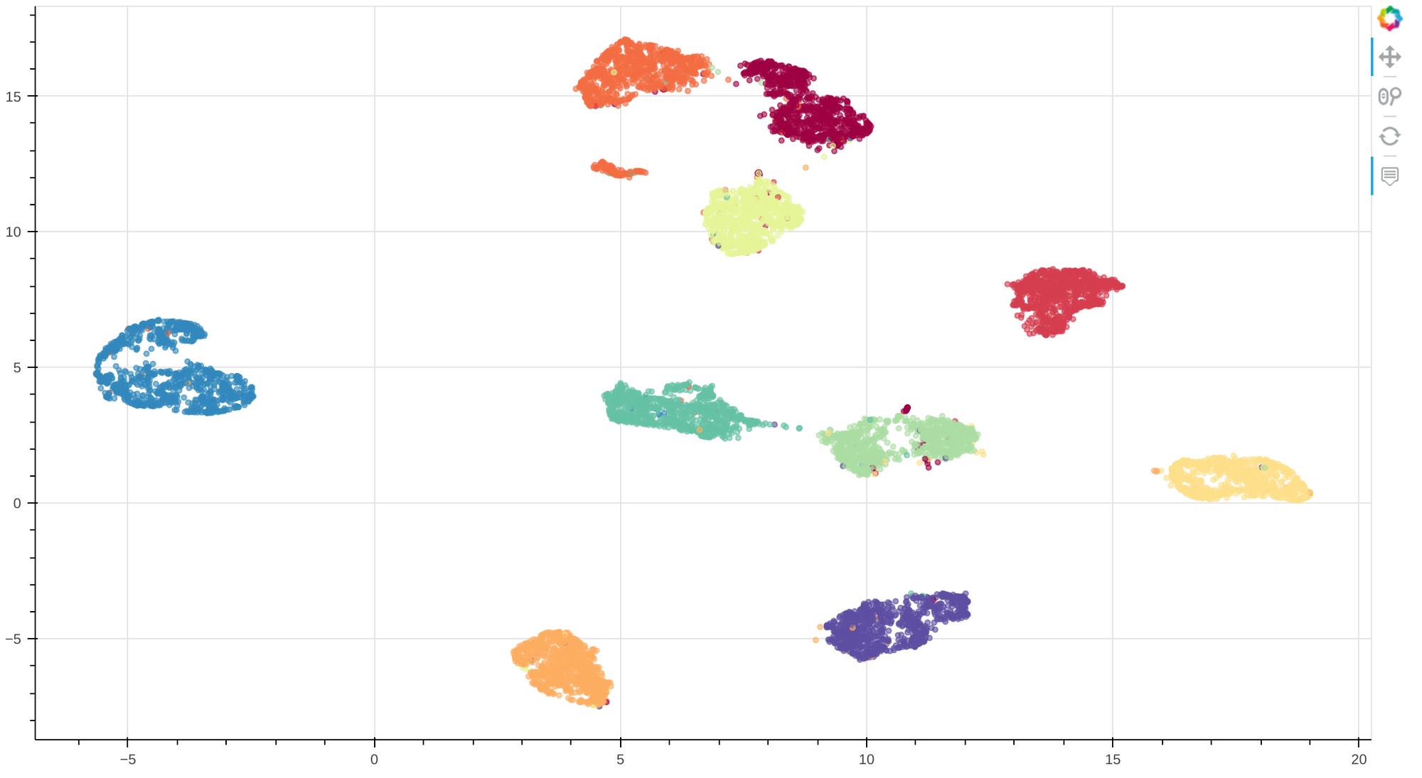
MNIST embeddings visualization. Each color represents a number from 0 to 9

This visualization demonstrates that there are clear clusters with few misassignments, supporting the statement that the model was able to learn a linearly separable (and thus disentangled) latent representation. A look at the interactive visualization suggests that most of the misassigned samples look very similar to the nearest ones. I especially like how crossed 7 forms a separate cluster, although this would cause problems if we wanted to label clusters.

CelebA and FFHQ

After testing the model on MNIST, it was trained on the CelebA + FFHQ datasets.

As before, let’s generate some random images to see if the model works correctly:

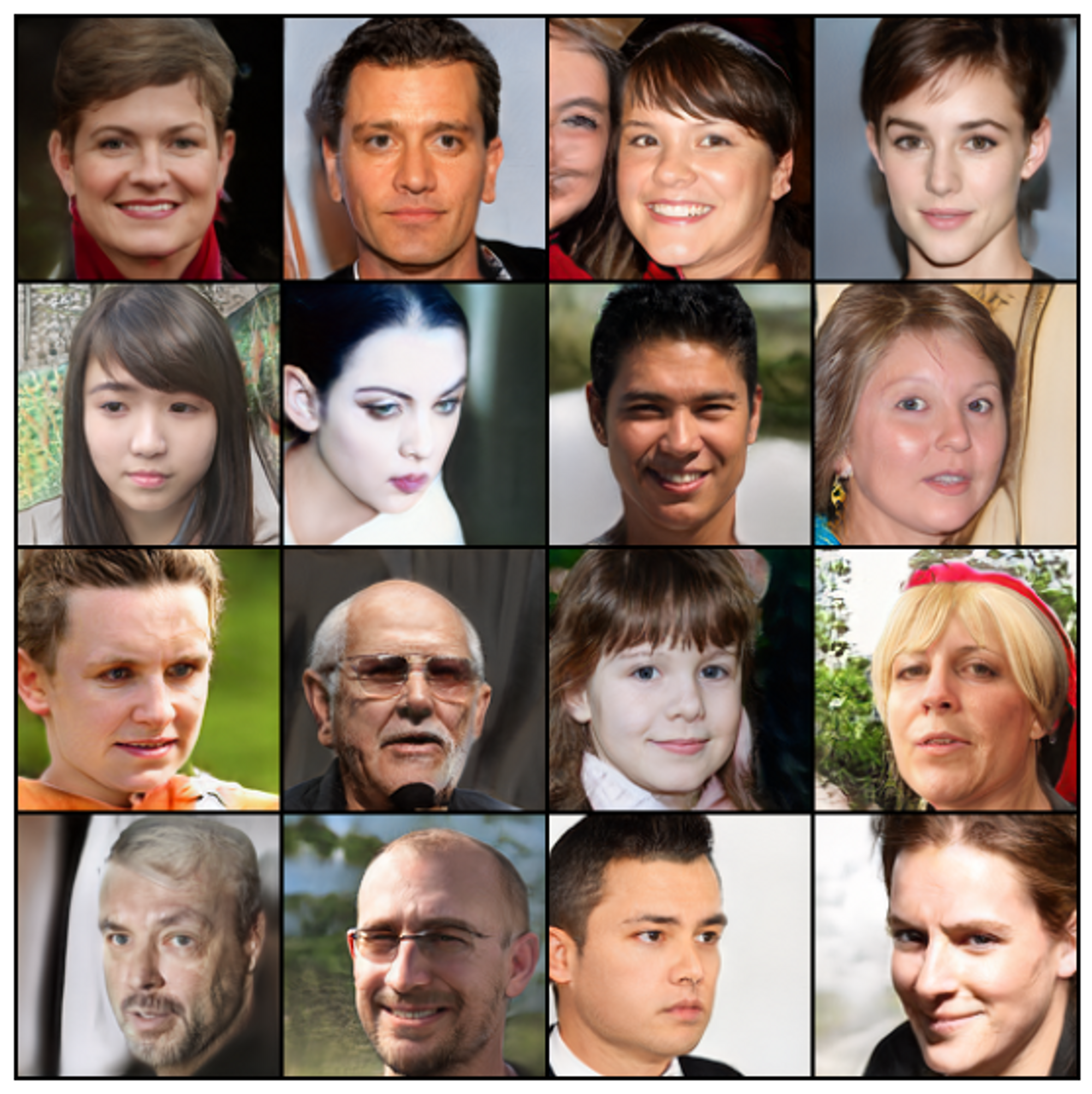
Synthetic images generated from noise using custom ALAE

Now, let’s reconstruct real images:

The first row represents original images, the second row demonstrates reconstruction

We can see that the images have been reconstructed inaccurately.

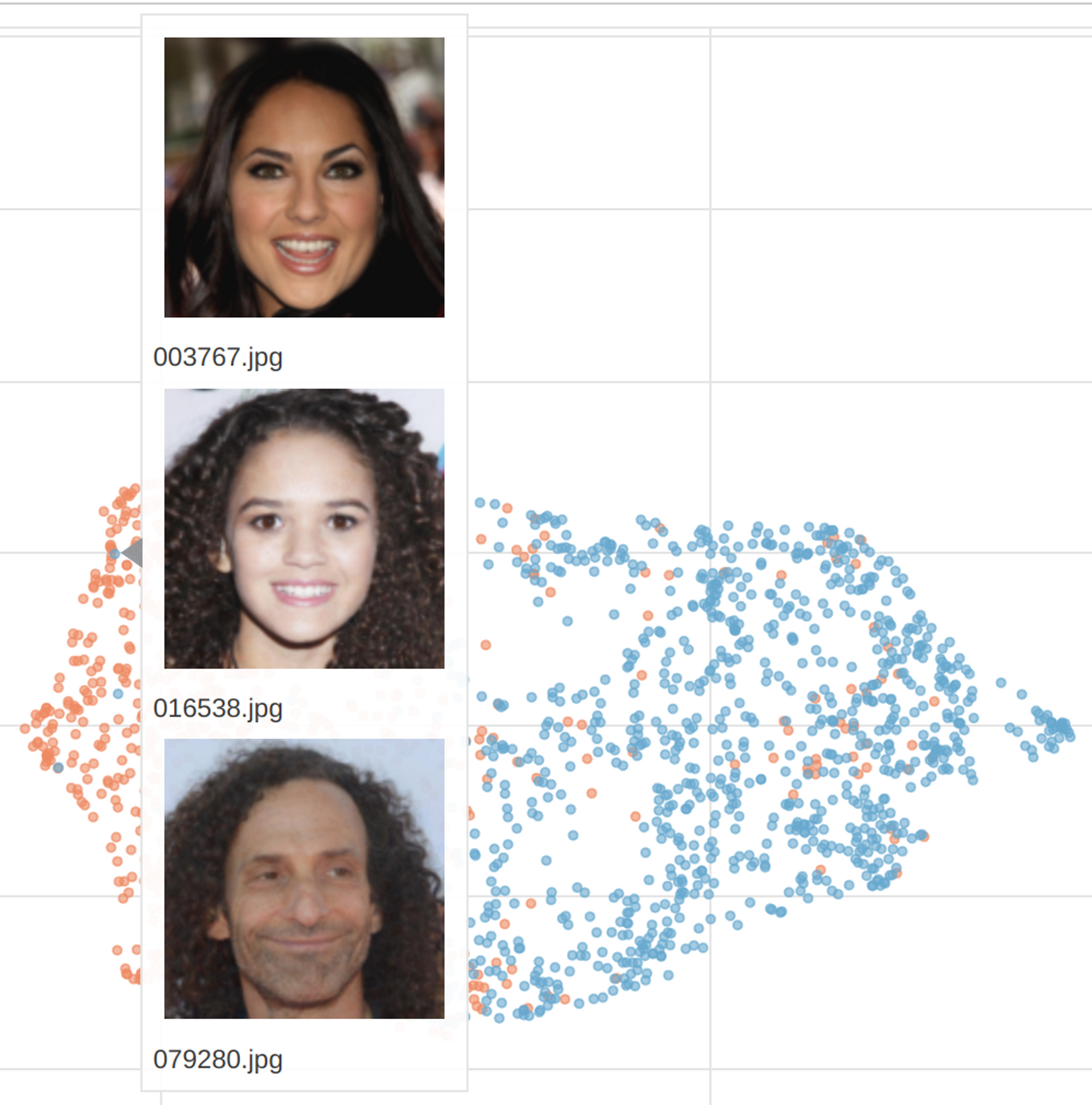
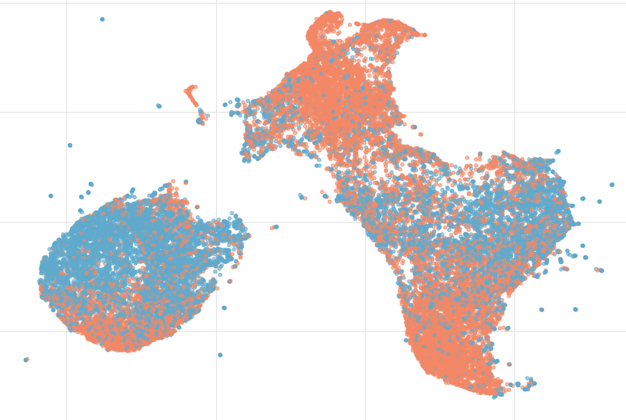
And here is a visualization of embedding with the gender attribute highlighted:

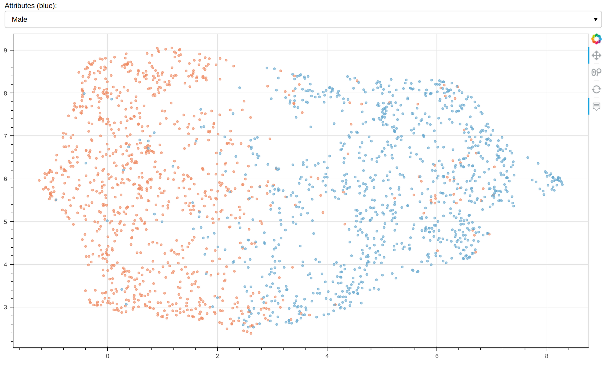
CelebA test set visualization of embeddings. Orange - female, blue - male.

At first glance, the model seems to have succeeded in capturing the gender attribute, but a closer look at the interactive visualization reveals that the haircut may play a greater role.

However, which features were decisive remains open. For instance, this diagram shows the attribute black hair:

black hair in blue

As previously mentioned, the reconstruction loss may decrease the quality of images. To test this, I added a reconstruction loss between real and generated images in pixel space. The figure below shows the results.

The first row shows real images; the second shows the reconstruction

The results confirm that optimizing a GAN in latent space is generally considered to be a better approach for image generation.

Camelyon

Finally, the model was trained on the Camelyon data set that consists of medical images of H&E-stained whole-slide images of lymph node sections containing normal tissues or with breast cancer metastases.

Similar to MNIST experiment, I trained linear SVM and logistic regression on the test set.

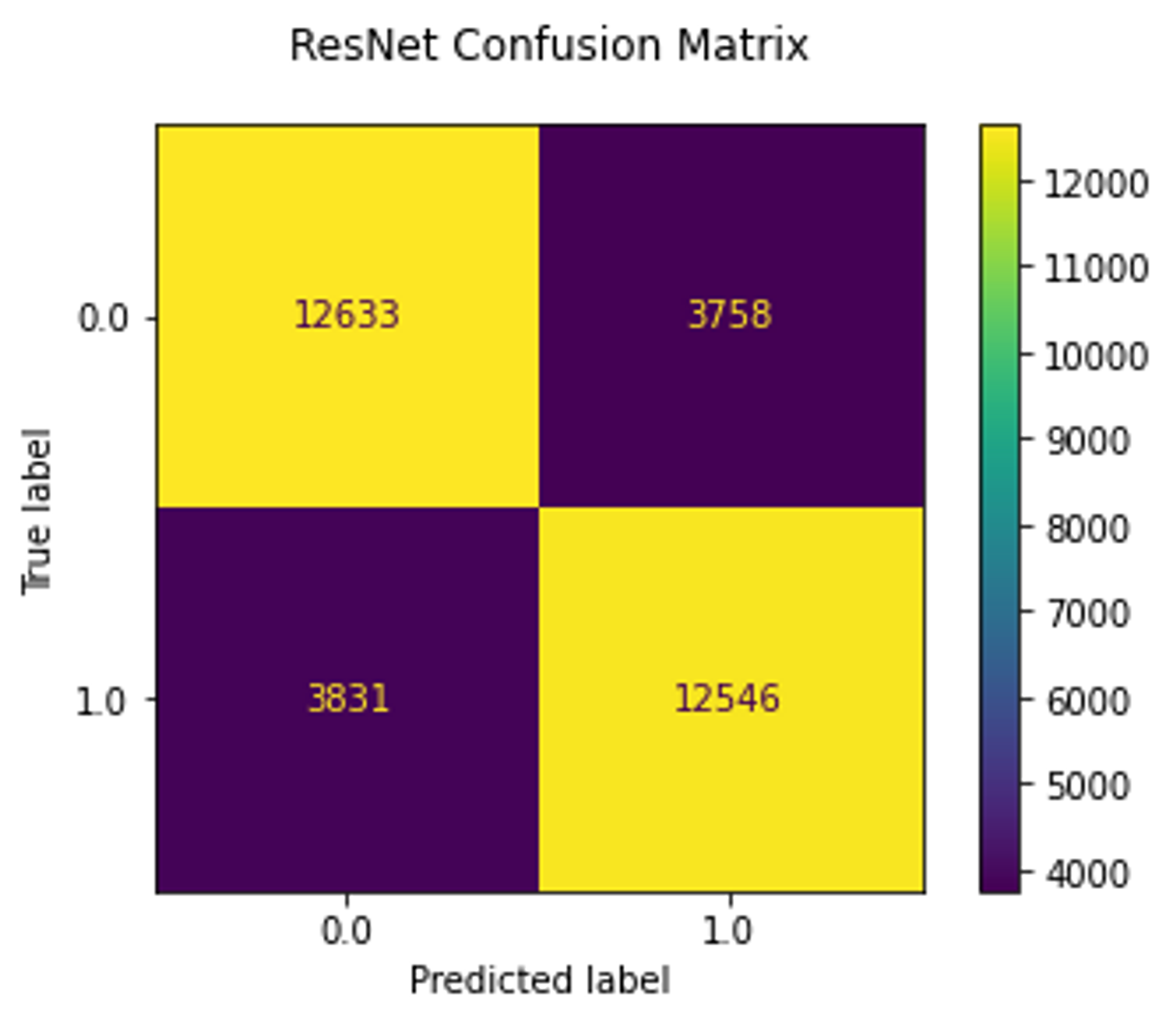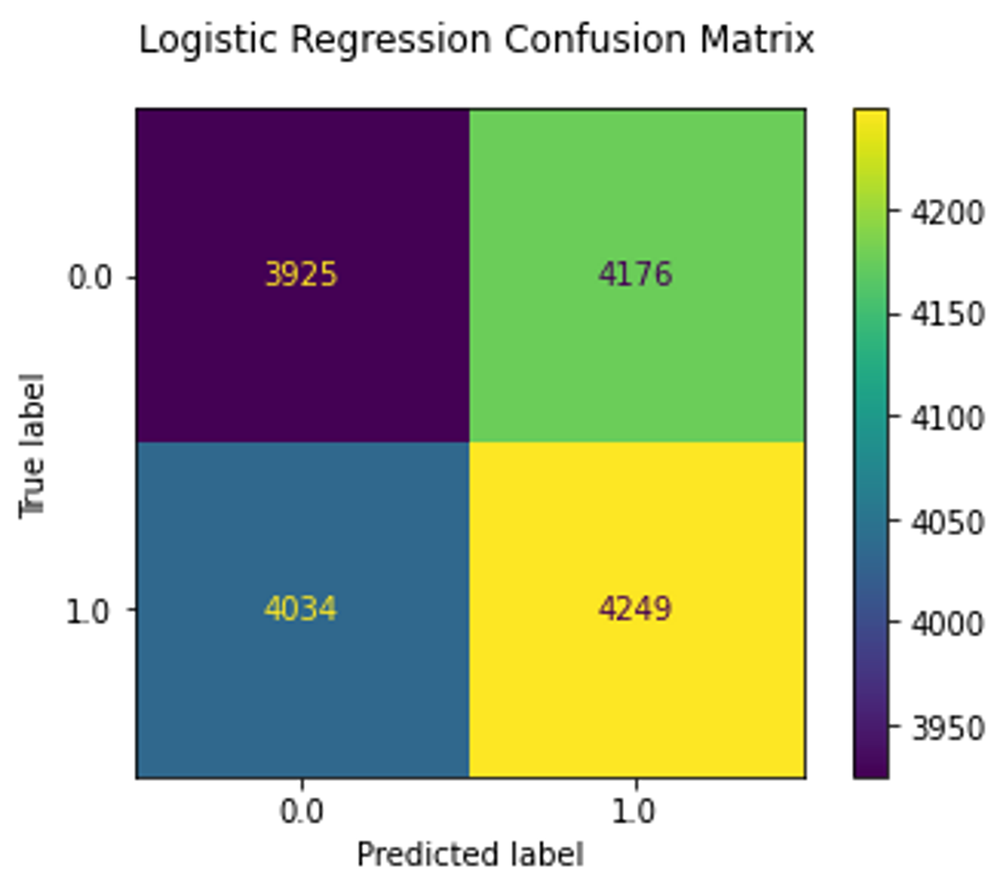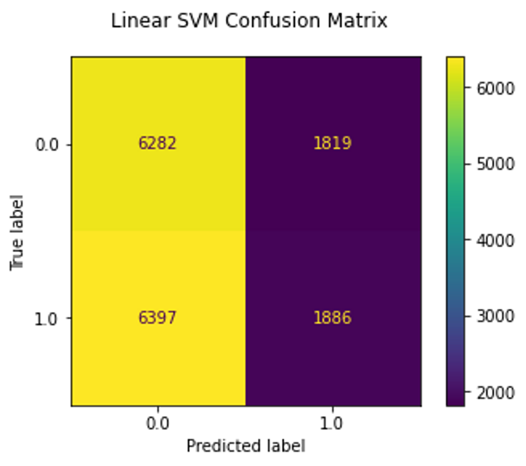As we can see, the ResNet18 model reached 77% accuracy, whereas linear models trained on embeddings reached only 50% which is a random choice.

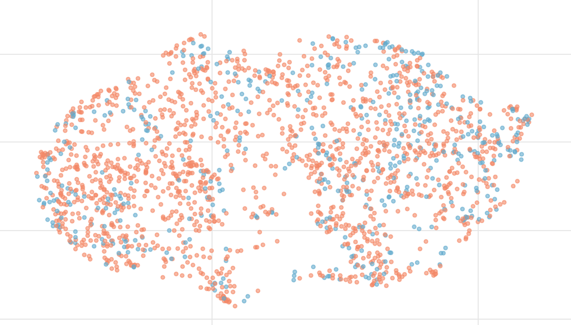
And here is a visualization of the embeddings:

This diagram shows embeddings colored by their class (normal, cancer). As you can see, these classes do not form clusters. This indicates that the model did not capture the cancer cells, making the approach useless for this dataset.

Note that there are several point clusters indicating that the dataset contains duplicates, completely black patches, and patches without tissues.

Conclusion

As we have just seen that decomposing and reusing the encoder part of the discriminator and adding a simple consistency loss allow real images to be projected into latent space. Having disentangled embeddings can potentially allow us to identify features in the latent space and assign semantical attributes to them, which may allow us to reason predictions in downstream tasks, assuming that the latent representation is indeed disentangled.

However, the linear separability of the embeddings does not necessarily mean that the latent representation is disentangled, nor does the visualization with UMAP. This question, therefore, remains open for further investigation. Nonetheless, we still can use embeddings to search for similar samples and, for example, clean and balance datasets.

Another issue is that the encoder approach is not optimal, causing the model to fail to accurately reconstruct images. There are already better methods for inverting real images, for instance, by combining the encoder approach and optimization technique, but it is also not optimal as we still need to run an iterative optimization until we get reasonable embeddings. I encourage you to watch this talk on the topic.

In conclusion, StyleGAN2 with encoder appears to be able to capture coarse details such as hair color or scanner color palette in digital pathology but may struggle with fine features that are only a few pixels in size. Further investigation is needed to confirm these findings.

References

[1] Karras, T., Laine, S., & Aila, T. (2018). A Style-Based Generator Architecture for Generative Adversarial Networks. arXiv

[2] Karras, T., Laine, S., Aittala, M., Hellsten, J., Lehtinen, J., & Aila, T. (2019). Analyzing and Improving the Image Quality of StyleGAN. arXiv

[3] Pidhorskyi, S., Adjeroh, D., & Doretto, G. (2020). Adversarial Latent Autoencoders. arXiv

[4] Wu, Zongze, Dani Lischinski, and Eli Shechtman. “Stylespace analysis: Disentangled controls for StyleGAN image generation.” Proceedings of the IEEE/CVF Conference on Computer Vision and Pattern Recognition. 2021. PDF